Download
1 / 36
360 likes | 500 Views
Chapter 3: Displaying and Describing Categorical Data. The Three Rules of Data Analysis. The three rules of data analysis won’t be difficult to remember: Make a picture —things may be revealed that are not obvious in the raw data. These will be things to think about.

E N D
The Three Rules of Data Analysis • The three rules of data analysis won’t be difficult to remember: • Make a picture—things may be revealed that are not obvious in the raw data. These will be things to think about. • Make a picture—important features of and patterns in the data will show up. You may also see things that you did not expect. • Make a picture—the best way to tell others about your data is with a well-chosen picture.
Frequency Tables • We can “pile” the data by counting the number of data values in each category of interest. • We can organize these counts into a frequency table, which records the totals and the category names.
Frequency Tables Example • What is your favorite color on this list? • Red • Blue • Green • Purple
Relative Frequency Tables • A relative frequency tableis similar, but gives the percentages (instead of counts) for each category. • Cumulative Frequency – calculates the sum of all relative frequencies for that particular category and all previous categories
Creating Frequency Tables • Both types of tables show how cases are distributed across the categories. • They describe the distributionof a categorical variable because they name the possible categories and tell how frequently each occurs. • To calculate the relative frequency: • Divide the count by the total number to cases • Multiply by 100 to express as a percentage • To calculate the cumulative relative frequency: • Take the current category’s relative frequency and add it all previous relative frequencies
Relative Frequency: Example • Let’s use the previous data we collected to create a relative frequency table.
What’s Wrong With This Picture? • You might think that a good way to show the Titanic data is with this display. Is it?
The Area Principle • The ship display makes it look like most of the people on the Titanic were crew members, with a few passengers along for the ride. • When we look at each ship, we see the area taken up by the ship, instead of the length of the ship. • The ship display violates the area principle: • The area occupied by a part of the graph should correspond to the magnitude of the value it represents.
Bar Charts • A bar chart displays the distribution of a categorical variable, showing the counts for each category next to each other for easy comparison. • A bar chart stays true to the area principle. • Thus, a better display for the ship data is: • Bar charts have spaces between the categories, while histograms do not.
Bar Charts (cont.) • A relative frequency bar chart displays the relative proportion of counts for each category. • A relative frequency bar chart also stays true to the area principle. • Replacing counts with percentages in the ship data:
How to Create Bar Charts • Use equal increments along the dependent (y) axis. • Follow the area principle and be sure to keep the area equal in each segment (the x-axis should also have equal increments). • Example: Create a bar graph based on the collected data:
Pie Charts • When you are interested in parts of the whole, a pie chart might be your display of choice. • Pie charts show the whole group of cases as a circle. • They slice the circle into pieces whose size is proportional to the fraction of the whole in each category.
How to Accurately Create Pie Charts • Convert Your Data: • Convert all data values to percentages of the whole data set. For example, four radishes, three cucumbers, two carrots and one pepper equals 40 percent radishes, 30 percent cucumbers, 20 percent carrots and 10 percent peppers. • Convert the percentages into angles. Since a full circle is 360 degrees, multiply this by the percentages to get the angle for each section of the pie. For the radishes, 0.4 X 360 = 144 degrees. For the cucumbers, 0.3 X 360 = 108 degrees. For the carrots, 0.2 X 360 = 72 degrees. For the peppers, 0.1 X 360 = 36 degrees. • Make sure the angle calculations are correct by adding all the angles. The total should be 360. 144 + 108 + 72 + 36 = 360. • You may be off by a tenth or so due to rounding, so be careful.
How to Accurately Create Pie Charts (cont.) • Draw the Chart: • Draw a circle on a blank sheet of paper, using a compass. While a compass is not necessary, using one will make the chart much neater and clearer by ensuring the circle is even. • Draw a radius, from the center to the right edge of the circle, using the ruler or straight edge. This will be the first base line. • Measure the largest angle in the data with the protractor, starting at the baseline, and mark it on the edge of the circle. Use the ruler to draw another radius to that point. Use this new radius as a base line for your next largest angle and continue this process until you get to the last data point. You will only need to measure the last angle to verify its value since both lines will already be drawn. • Label and shade the sections of the pie chart to highlight whatever data is important for your use.
Day 2 Class Activity • What’s your favorite academic subject? • Create your own pie chart to represent the class’s distribution of subject preferences.
Contingency Tables • A contingency table allows us to look at two categorical variables together. • It shows how individuals are distributed along each variable, depending on the value of the other variable. • Example: we can examine the class of ticket and whether a person survived the Titanic:
Contingency Tables (cont.) • The margins of the table, both on the right and on the bottom, give totals and the frequency distributions for each of the variables. • Each frequency distribution is called a marginal distribution of its respective variable. • The marginal distribution of Survival is:
Contingency Tables (cont.) • Each cellof the table gives the count for a combination of values of the two values. • For example, the second cell in the crew column tells us that 673 crew members died when the Titanic sunk.
Contingency Table Example • The percentage of passengers who were both in 1st class and survived: • The percentage of 1st class passengers who survived: • The percentage of the survivors who were in 1st class: • Contingency tables allow us to make many comparisons.
Example: Finding Marginal Distributions • This two-way table shows the favorite leisure activities for 50 adults - 20 men and 30 women. • What is the marginal distribution of the responses?
Conditional Distributions • A conditional distribution shows the distribution of one variable for just the individuals who satisfy some condition on another variable. • The following is the conditional distribution of ticket Class, conditional on having survived:
Conditional Distributions (cont.) • The following is the conditional distribution of ticket Class, conditional on having passed:
Conditional Distributions (cont.) • The conditional distributions tell us that there is a difference in class for those who survived and those who perished. • This is better shown with pie charts of the two distributions:
Conditional Distributions (cont.) • We see that the distribution of Class for the survivors is different from that of the nonsurvivors.. • This leads us to believe that Class and Survival are associated, that they are not independent. • The variables would be considered independentwhen the distribution of one variable in a contingency table is the same for all categories of the other variable.
Activity: Political Views • What % of the class are girls with liberal political views? • What % of conservatives are boys? • What % of girls are moderate? • What is the marginal frequency distribution of political views? • What is the conditional distribution of gender among conservatives?
Day 3 Simpson’s Paradox • When averages are taken across different groups, they can appear to contradict the overall averages.
Simpson’s Paradox (cont.) • It’s the last inning of an important game. Your team is one run down with the bases loaded and two outs. The pitcher is due up, so you’ll be sending in a pinch-hitter. There are two batters available on the bench. Whom should you send in to bat? • Do the averages line up with the overall?
Segmented Bar Charts • A segmented bar chart displays the same information as a pie chart, but in the form of bars instead of circles. • Each bar is treated as the “whole” and is divided proportionally into segments corresponding o the percentage in each group. • Here is the segmented bar chart for ticket Class by Survival status:
What Can Go Wrong? • Don’t violate the area principle. • While some people might like the pie chart on the left better, it is harder to compare fractions of the whole, which a well-done pie chart does.
What Can Go Wrong? (cont.) • Keep it honest—make sure your display shows what it says it shows. • This plot of the percentage of high-school students who engage in specified dangerous behaviors has a problem. Can you see it?
What Can Go Wrong? (cont.) • Don’t confuse similar-sounding percentages—pay particular attention to the wording of the context. • Don’t forget to look at the variables separately too—examine the marginal distributions, since it is important to know how many cases are in each category.
What Can Go Wrong? (cont.) • Be sure to use enough individuals! • Do not make a report like “We found that 66.67% of the rats improved their performance with training. The other rat died.”
What Can Go Wrong? (cont.) • Don’t overstate your case—don’t claim something you can’t. • Don’t use unfair or silly averages—this could lead to Simpson’s Paradox, so be careful when you average one variable across different levels of a second variable.
Recap • We can summarize categorical data by counting the number of cases in each category (expressing these as counts or percents). • We can display the distribution in a bar chart or pie chart. • And, we can examine two-way tables called contingency tables, examining marginal and/or conditional distributions of the variables.
Assignments: pp. 38-39 • Day 1: #5 – 9 ODD, 11, 13 – 16 • Day 2: # 17, 19 – 21 • Day 3: # 23, 25, 28 • Day 4: # 32, 33, 39 • Read Chapter 4