Download

1 / 57
570 likes | 694 Views
Characterizing CO 2 fluxes from oceans and terrestrial ecosystems. Nir Krakauer PhD thesis seminar May 19, 2006. The atmospheric CO 2 mixing ratio. Australian Bureau of Meteorology. Warming is underway. Dragons Flight (Wikipedia) Data: Hadley Centre .

E N D
Characterizing CO2 fluxes from oceans and terrestrial ecosystems Nir Krakauer PhD thesis seminar May 19, 2006
The atmospheric CO2 mixing ratio Australian Bureau of Meteorology
Warming is underway Dragons Flight (Wikipedia) Data: Hadley Centre
The atmospheric CO2 mixing ratio:A closer look • 1990s fossil fuel emissions: 6.4 Pg carbon / year • The amount of CO2 in the atmosphere increased by 3.2 Pg C / year • Where did the other half of the CO2 go? • Why the interannual variability?
Ocean CO2 uptake • The ocean must be responding to the higher atmospheric pCO2; models estimate ~2 Pg C/ year uptake • Hard to measure directly because air-sea CO2 fluxes are patchy, depending on ocean circulation, biology, heating, gas exchange rate LDEO
CO2 uptake on land Buermann et al 2002 • Change in C content of biomass very patchy; hard to extrapolate from small-scale surveys… • Uptake must make up for ~1.5 Pg C / year deforestation • Land biomass might be growing because of longer growing seasons, CO2 fertilization, N fertilization, fire suppression, forest regrowth…
1) Tree-ring evidence for the effect of volcanic eruptions on plant growth Chris Newhall, via GVP Henri D. Grissino-Mayer N. Y. Krakauer, J. T. Randerson, Global Biogeochem. Cycles17, doi: 10.1029/2003GB002076 (2003)
Motivation • Why did the atmospheric CO2 growth rate drop for 2 years after the 1991 Pinatubo eruption? • Changes in the latitudinal CO2 gradient and in δ13C suggest that part of the sink was from northern land biota • An enhanced carbon sink also followed the 1982 El Chichón and 1963 Agung eruptions
How would eruptions lead to a carbon sink? • Roderick et al (2001) and Gu et al (2003): light scattering by aerosols boosts canopy photosynthesis for 1-2 years after eruptions • Jones and Cox (2001) and Lucht et al (2002): soil respiration is lower because of cooling; boreal photosynthesis decreases Gu et al 2003 Harvard Forest (clear skies) Lucht et al 2002
What I did • What happened to tree ring widths after past eruptions? • Large eruptions since 1000 from ice core sulfate time series • 40,000 ring width series from the International Tree Ring Data Bank (ITRDB) Crowley 2000
Part 1: Conclusions • Northern trees (>45°N) had narrower rings up to 8 years after Pinatubo-size eruptions • Eruptions had no significant effect on trees at other latitudes (few trees from the tropics though) • From this sample, negative influences on NPP appear to dominate positive ones –respiration slowdown is likely to be responsible for the inferred carbon sink
Part 1: Research directions • Are there niches where diffuse light does strongly enhance growth? – understory trees, tropical rainforest… • Why are boreal rings narrower so long after eruptions? • Can we tell what happens to trees’ physiology after eruptions (short growing season, nutrient stress…)? – tree-ring δ13C, δ15N
2) Selecting parameters in inversions for regional carbon fluxes by generalized cross-validation Baker et al 2006 N. Y. Krakauer, T. Schneider, J. T. Randerson, S. C. Olsen, Geophys. Res. Lett.31, doi: 10.1029/2004020323 (2004).
CO2 fluxes from concentration differences: a linear inverse problem Measurements of CO2 concentrations, with error covariance matrix Cb the (unknown) flux magnitudes Ax ≈ b A transport operator that relates concentration patterns to flux magnitudes x ≈ x0 A plausible prior flux distribution, with prior uncertainty covariance matrix Cx
Ambiguities in parameter choice • Solving the inverse problem requires specifying Cb, Cx, x0 • Adjustable parameters include: How much weight to give the measurements vs. the prior guesses? Weight CO2 measurements equally or differentially? • Different parameter values lead to varying results for, e.g., the land-ocean and America-Eurasia distribution of the missing carbon sink
Generalized cross-validation (GCV) • Craven and Wahba (1979): a good value of a regularization parameter in an inverse problem is the one that provides the best invariant predictions of left-out data points • Choose the parameter values that minimize the “GCV function”: T = effective degrees of freedom GCV=
The TransCom 3 inversion • Estimates mean-annual fluxes from 11 land and 11 ocean regions • Data: 1992-1996 mean CO2 concentrations at 75 stations, and the global mean rate of increase Gurney et al 2002
Parameters varied • λ: How closely the solution would fit the prior guess x0 • controls size of the prior-flux variance Cx • higher λ: solution will be closer to x0 (more regularization) • Weighting used in original TransCom inversion taken as λ=1 • τ: How much preference to give data from low-variance (oceanic) stations • controls structure of the data variance Cb • 0: all stations weighted equally • TransCom value: 1
Results: the GCV function Function minimum Parameter values used in TransCom
overall inferred flux distribution TransCom parameter values GCV parameter values
(2) Conclusion and research directions • Parameter choice explains part of the variability in CO2 flux estimates derived from inverse methods • GCV looks promising for empirically choosing parameter values in global-scale CO2 inversions, e.g. weights for different types of information • GCV-based parameter choice methods should also be useful for studies that try to solve for carbon fluxes at high resolution (e.g. NACP)
3) Regional air-sea gas transfer velocities estimated from ocean and atmosphere carbon isotope measurements GasEx N. Y. Krakauer, J. T. Randerson, F. W. Primeau, N. Gruber, D. Menemenlis, submitted to Tellus
A conceptual model of gas exchange: the stagnant film • Most of the air-sea concentration difference is across a thin (<0.1 mm) water-side surface layer • F = kw (Cs – Ca) • F: gas flux (mass per surface area per time) • Cs: gas concentration in bulk water (mass per volume) • Ca: gas concentration in bulk air (partial pressure * solubility) • kw: gas transfer coefficient (a “gas transfer velocity”) 100 μm J. Boucher, Maine Maritime Academy
Measured gas transfer velocities range widely… • Gas transfer velocity usually plotted against windspeed (roughly correlates w/ surface turbulence) • Many other variables known/theorized to be important: wave development, surfactants, rain, air-sea temperature gradient… • Several measurement techniques have been used – all imprecise, sometimes seem to give systematically different results Wu 1996; Pictures: WHOI • What’s a good mean transfer velocity to use?
..as do parameterizations of kw versus windspeed • Common parameterizations assume kw to increase with windspeed v (piecewise) linearly (Liss & Merlivat 1986), quadratically (Wanninkhof 1992) or cubically (Wanninkhof & McGillis 1999) • Large differences in implied kw, particularly at high windspeeds (where there are few measurements) • Are these formulations consistent with ocean tracer distributions? Feely et al 2001
CO2 isotope gradients are excellent tracers of air-sea gas exchange • Because most (99%) of ocean carbon is ionic and doesn’t directly exchange, air-sea gas exchange is slow to restore isotopic equilibrium • Thus, the size of isotope disequilibria is uniquely sensitive to the gas transfer velocity kw ppm Sample equilibration times with the atmosphere of a perturbation in tracer concentration for a 50-m mixed layer μmol/kg Ocean carbonate speciation(Feely et al 2001)
Optimization scheme Assume that kw scales with some power of climatological windspeed u: kw = <k> (un/<un>) (Sc/660)-1/2, (where <> denotes a global average, and the Schmidt number Sc is included to normalize for differences in gas diffusivity) find the values of <k>, the global mean gas transfer velocity and n, the windspeed dependence exponent that best fit carbon isotope measurements using transport models to relate measured concentrations to corresponding air-sea fluxes
Windspeed varies by latitude SSM/I climatological wind (Boutin and Etcheto 1996)
The radiocarbon cycle at steady state • 14C (λ1/2 = 5730 years) is produced in the upper atmosphere at ~6 kg / year • Notation: Δ14C = 14C/12C ratio relative to the preindustrial troposphere Stratosphere+80‰ 90 Pg C 14N(n,p)14C Troposphere0‰ 500 Pg C Land biota–3‰ 1500 Pg C Air-sea gas exchange Shallow ocean –50‰ 600 Pg C Deep ocean–170‰ 37000 Pg C Sediments–1000‰ 1000000 Pg C
The bomb spike: atmosphere and surface ocean Δ14C since 1950 • Massive production in nuclear tests ca. 1960 (“bomb 14C”) • Through air-sea gas exchange, the ocean took up ~half of the bomb 14C by the 1980s data: Levin & Kromer 2004; Manning et al 1990; Druffel 1987; Druffel 1989; Druffel & Griffin 1995 bomb spike
Ocean bomb 14C uptake: previous work • Broecker and Peng (1985; 1986; 1995) used 1970s (GEOSECS) measurements of 14C in the ocean to estimate the global mean transfer velocity, <k>, at 21±3 cm/hr • This value of <k> has been used in most subsequent parameterizations of kw(e.g. Wanninkhof 1992) and for modeling ocean CO2 uptake • Based on trying to add up the bomb 14C budget, suggestions have been made (Hesshaimer et al 1994; Peacock 2004)are that Broecker and Peng overestimated the ocean bomb 14C inventory, so that the actual value of <k> might be lower by ~25%
Ocean 14C goals • From all available (~17,000) ocean Δ14C observations, re-assess the amount of bomb 14C taken up, estimate the global mean gas transfer velocity, and bound how it varies by region • The 1970s (GEOSECS) observations plus measurements from more recent cruises (WOCE) data: Key et al 2004
Modeling ocean bomb-14C uptake • Simulate ocean uptake of bomb 14C (transport fields from ECCO-1°), given the known atmospheric history, as a function of the air-sea gas transfer velocity • Find the air-sea gas transfer velocity that best fits observed14C levels
Results: simulated vs. observed bomb 14C by latitude – 1970s • For a given <k>, high n leads to more simulated uptake in the Southern Ocean, and less uptake near the Equator • Observation-based inventories seem to favor low n (i.e. kw increases slowly with windspeed) Simulations for <k> = 21 cm/h and n = 3, 2, 1 or 0 Observation-based mapping (solid lines) from Broecker et al 1995; Peacock 2004
Simulated-observed ocean 14C misfit as a function of <k> and n • The minimum misfit between simulations and (1970s or 1990s) observations is obtained when <k> is close to 21 cm/hr and n is low (1 or below) • The exact optimum <k> and n change depending on the misfit function formulation used (letters; cost function contours are for the A cases) , but a weak dependence on windspeed (low n) is consistently found
Optimum gas transfer velocities by region • As an alternative to fitting <k> and n globally, I estimated the air-sea gas exchange rate separately for each region, and fit <k> and n based on regional differences in windspeed • Compared with previous parameterizations (solid lines), found that kw is relatively higher in low-windspeed tropical ocean regions and lower in the high-windspeed Southern Ocean (+s and gray bars) • Overall, a roughly linear dependence on windspeed (n ≈ 1; dashed line)
Simulated mid-1970s ocean bomb 14C inventory vs. <k> and n • The total amount taken up depends only weakly on n, so is a good way to estimate <k> • The simulated amount at the optimal <k> (square and error bars) supports the inventory estimated by Broecker and Peng (dashed line and gray shading)
Other evidence: atmospheric Δ14C °N • I estimated latitudinal differences in atmospheric Δ14C for the 1990s, using observed sea-surface Δ14C, biosphere C residence times (CASA), and the atmospheric transport model MATCH • The Δ14C difference between the tropics and the Southern Ocean reflects the effective windpseed dependence (n) of the gas transfer velocity
Observation vs. modeling • The latitudinal gradient in atmospheric Δ14C (dashed line) with the inferred <k> and n, though there are substantial uncertainties in the data and models (gray shading) • More data? (UCI measurements) • Similar results for preindustrial atmospheric Δ14C (from tree rings) • Also found that total ocean 14C uptake preindustrially and in the 1990s is consistent with the inferred <k> <k> (cm/hr) n (‰ difference, 9°N – 54°S)
14C conclusions • The power law relationship with the air-sea gas transfer velocity kw that best matches observations of ocean bomb 14C uptake has • A global mean <k>=21±2 cm/hr, similar to that found by Broecker and Peng • A windspeed dependence n= 0.9±0.4 (about linear), compared with 2-3 for quadratic or cubic dependences • This is consistent with other available 14C measurements
The ocean is now releasing 13C to the atmosphere… 1977-2003 • Notation – δ13C: 13C/12C ratio relative to a carbonate standard • The atmospheric 13C/12C is steadily declining because of the addition of fossil-fuel CO2 with low δ13C; this fossil-fuel CO2 is gradually entering the ocean Scripps (CDIAC)
…and the amount can be estimated… PgC∙‰ carbon-13 • Budget elements • the observed δ13C atmospheric decline rate (arrow 1) • biosphere disequilibrium flux (related to the carbon residence time) (5) • fossil fuel emissions (6) • biosphere (4) and ocean (2) net carbon uptake (apportioned using ocean DIC measurements) • I calculated that air-sea exchange must have brought 70±17 PgC∙‰ 13C to the atmosphere in the mid-1990s, ~half the depletion attributable to fossil fuels Pg carbon Randerson 2004
…but the air-sea δ13C disequilibrium is of opposite sign at low vs. high latitudes Sea-surface δ13C (‰) • Reflects fractionation during photosynthesis + temperature-dependent carbonate system fractionation • The dependence of kw on windspeed must yield the inferred global total flux Air-sea δ13C disequilibrium (‰) data: GLODAP (Key 2004) Temperature-dependent air-sea fractionation (‰)