Download

1 / 54
540 likes | 704 Views
Investigating trap catches using the Diffusion process and individual stochastic based models. Danish Ali Ahmed daa11@le.ac.uk Leicester University 2012 (Supervisor: Dr. Sergei Petrovskii ) . CONTENTS. Section 1 Introduction to pest trapping

E N D
Investigating trap catches using the Diffusion process and individual stochastic based models. Danish Ali Ahmed daa11@le.ac.uk Leicester University 2012 (Supervisor: Dr. Sergei Petrovskii)
CONTENTS • Section 1 • Introduction to pest trapping • Modelling of movement and the Diffusion process • Finite Difference method – Explicit/Implicit scheme • Mean field approach • Individual based model • Circular field with a circular trap installed at the centre (MFA) • Square field with a circular trap installed at the centre (IBM) • Comparison between MFA and IBM under similar geometry • Stochastic Fluctuations • Conclusion
CONTENTS • Section 2 • The 2-D Diffusion equation and the flux of the system • The cross shaped trap • Investigating the effect of the position of an initial point source release on trap catches • Modelling Click Beetle (Agriotesobscurus, Females) trap catches • Other research work (Some listed problems)
Section 1: 1) Introduction to pest trapping • An essential component of monitoring integrated pest management programmes is the trapping of insects. • There are mainly two types of traps commonly used in the research field of ecological studies and pest management. These are passive and baited traps. Passive trapping relies on the movement of individual insects into a capturing zone whereas baited traps lure the insects through the usage of an attractant. • We will be interested in passive traps. • Scientists have regularly used passive traps to monitor populations. The most common approaches include the ’mark-release-capture’ method and the other uses the concept of counts as density measures. • The main aim is to construct a comprehensive understanding and interpretation of trap counts, with a well defined and consistent mathematical framework.
Over the last two decades research has been directed towards the study of movement, however mathematicians still lack a consistent framework for the modelling of such a phenomenon. This is not due to neglect of such a notion, however it is known that the study of movement is intrinsically difficult since it consists of at least two scales - temporal and spatial. • Once passive trapping is well understood we can investigate more complicated systems which incorporate wind effects and also baited trapping with an attractant (food/lighting). • A natural extension would lead to the study of multiple traps. • Common models include discrete individual based models (Lagrangian viewpoint) and Diffusion processes (Eulerian viewpoint).
2) Modelling of movement and the Diffusion process • Two main conceptual approaches assigned to the modelling of movement. • The Lagrangian and the Eulerian viewpoint. • Lagrangian point of view concentrates on the moving individual. Includes the characterization of velocity, acceleration, turning angles . . . • Eulerian models are characterized by population densities and fluxes at spatial points. • Diffusion models are examples of Eulerian models. • Individual based models (IBM) are considered as Lagrangian models.
Both Lagrangian and Eulerian models complementeachother. • The Diffusion process is the process by which matter is transported from one part of a system to another as a result of random particle motion. • The motion of particles is completely random, independent and isotropic. • The fundamental idea of Diffusion is based on the Fickian hypothesis.
Fickian hypothesis: Rate of transfer of diffusive substance through a unit area of a section is proportional to the concentration gradient measured normal to the section F = rate of transfer per unit area of cross section. u = Concentration of diffusing substance. x = Spatial co-ordinate measured normal to the section. D = Diffusion coefficient.
Once derived (See crank 1975) we obtain the Diffusion equation Or more generally in n dimensions. • We will be interested in the 1D and 2D Diffusion equations. where D = D(t) is possibly time dependent.
3) Finite difference method. • An analytic solution cannot always be found for the Diffusion equation provided an initial condition and suitable boundary conditions. • We resort to the discretization of the geometry and solve the system numerically using finite difference methods. • The 1D Diffusion equation with constant diffusion coefficient can be formally discretized using the differencing technique.
The finite difference method (Explicit and Implicit) • is the parameter which distinguishes different schemes with • (Spatial step) • (Time step)
Explicit scheme • Explicit method is known to be numerically stable and convergent provided the courant condition is satisfied. • Numerical error:
Implicit scheme • Scheme is always numerically stable and convergent. • More numerically intensive than the explicit method. • Requires solving a system of numerical equations in each time step. • Numerical error:
4) Mean field approach (MFA). • Consider the 1D Diffusion equation with constant diffusion coefficient • Initial condition: Initial population density • Boundary condition: • Using the explicit scheme the governing equation becomes with
Discretization of (Initial/Boundary) conditions: • Initial condition: • Boundary condition at x = 0,L:
5) Individual based model (IBM). • Alternative way to look at the dynamics of trap counts is to simulate the movement of each individual in the field (Lagrangian viewpoint). • Particle moves under curvilinear track • Observations allow recording at certain moments, correspondingly the curvilinear path is mapped into a series of broken lines • Time step • Assume Increment in time is constant.
Individual at a position at time will be at position at time • The movement vector can be described by in rectangular / polar co-ordinates respectively. is the step length and the turning angle. • or are random variables, therefore the movement is a stochastic process. • Assume no correlation between two subsequent steps • Statistical properties of movement are independent of time. • Process is essentially Markov, i.e A process with no memory. Each subsequent step does not carry any information based on the previous step.
The properties of the movement are fully determined by the probability distribution functions for and We denote these distributions as and respectively. • Model the increments to be Gaussian (Normally distributed) where are the variances. • Environment is isotropic, no advection and no drift. • The signature of the process is that the mean squared displacement is proportional to time i.e mean squared displacement grows linearly with time
Recall that we stated that both Eulerian and Langrangian viewpoints complement eachother. • This agreement is formed using the signature of the process i.e a relation between Diffusion coefficient and the variance. • Provided that D is fixed and is fixed
6) 2D: Circular field with a circular trap installed at the centre (MFA) • Solve the Diffusion equation in polar coordinates. • The population of the species u(r,t) is to be radially symmetric and axisymmetric. • Consider the following problem: BC’s: on on IC:
We calculate the flux of the system • Use finite difference method (explicit scheme) to solve the problem numerically. • Use numerical integration to evaluate the flux curve K(t).
7) 2D: Square field with a circular trap installed at the centre (IBM) • Consider a square field with dimensions • Install a circular trap at the centre of the field with radius • Step lengths are normally distributed in both the x and y directions with variance • If an individual particle falls into the trap then it is removed from the system • The far field boundary acts as a reflective boundary • To ensure that individuals which reach the far field do not influence the trap counts we require that
Additional comments for comparison between MFA and IBM We require the following in order to compare the MFA and IBM: • Typical lengths in the field are large in comparison to the typical length of the trap • Recall: • To reduce stochastic fluctuations we can increase the no. Of individual particles introduced initially. For fixed field area this refers to an increase in population density • We expect a smoother transition of influx as we increase
8) Comparison between MFA and IBM under similar geometry. Fix the following parameters: • Constant Diffusion coefficient: • Length of square field: • Time increment for IBM: • Number of particles for IBM and MFA: Calculated parameters: • MSD: • Field area must be the same: • Error in Field area:
9) Stochastic fluctuations • Let represent the flux of the particles in the IBM at time step • Let represent the flux of the particles in the mean field approach over some time interval
How do we reduce these stochastic fluctuations? • Define the relative maximum of the stochastic fluctuations as
Tabulated values which illustrate the smooth transition of influx as we increase
10) Conclusion • Successfully compared the individual based model and the mean field approach, used for the trapping of insects. Calculated a theoretical value for δ. • Both processes essentially govern the dynamics of the pests • Both Eulerian and Lagrangian methods complement each other Some discussion points: • Can we use these processes to describe or simulate pest trapping in the field? • If yes, can we find an analytical solutions for simple cases or simple geometries? • If no, can we enhance the models described to incorporate real motion in the field? • Super diffusive processes? Levy flights?
CONTENTS • Section 2 • The 2-D Diffusion equation and the flux of the system • The cross shaped trap • Investigating the effect of the position of an initial point source release on trap catches • Modelling Click Beetle (Agriotesobscurus, Females) trap catches • 1D Analytic solution via the Greens function for Super Diffusion • Introduction of Levy flights via the Cauchy distribution as opposed to Brownian motion • Matching Super diffusive flux curves to flux curves produced by Cauchy distributed step lengths • Further research • Other research work (Some listed problems)
1) The 2D Diffusion equation and the flux of the system • The 2D Diffusion equation • Flux of the system is defined in general as where is the trap boundary, is a normal vector to the trap boundary.
The 2D Diffusion equation will be solved numerically using the explicit finite difference technique. The flux will be evaluated using numerical integration. The initial condition. • The most common design for studying dispersal is the instantaneous point source release, in which marked organisms are released instantaneously at one point in time (usually t = 0) at a single point in space. • Formally this is described using the dirac delta function
For the IBM we place N particles at a fixed position • For the MFA it is not so straight forward. We model the point source release using an initial Gaussian profile • We must ensure that is not too small i.e on the order of the mesh step size Nor should it be too large as the wide spread of the profile will not reflect the PSR.
2) The cross shaped trap • A cross shaped trap is installed at the centre of a field of length with absorbing boundaries. • The cross shaped trap has wing length and tip length with fixed perimeter • We introduce an initial point source release at a distance from the centre of the cross subtending an angle from the horizontal wing. ε r ϒ θ L L
We model the spatio-temporal motion of the pests using the Diffusion equation with the initial standard bi-variate Gaussian distribution. • We investigate how the orientation and radial distance of the point source release effects the trap catches.
EVOLUTION: The evolution of the two dimensional Gaussian distribution for fixed r = 6, θ = π/4 and times t = 0.5, 1.5, 2.5 and 2.9 days.
CLOSE UP: A ‘close up’ of the point source release for fixed r = 6, θ = π/4 and time t = 2.9 days in the vicinity of the trap.
3) Investigating the effect of the position of an initial PSR on trap catches The effect on trap catches for varying radial distance and fixed orientation θ = π/4as time evolves.
The effect of orientation on trap catches for varying radial distance at fixed time t = 1.5 days.
The effect of radial distance on trap catches for varying orientation and fixed time t = 1.5 days
Obtain a monotonously decreasing dependency of flux on radial distance, i.e the further the point source release from the centre of the cross shaped trap, the lower the trap counts. • The optimal trap counts are obtained at θ = π/8,3π/8 from the values of θ investigated. A clear indication that individuals that approach the trap from these angles have a greater chance of being trapped. • Individuals that approach the trap from a horizontal (θ = 0) or vertical (θ = π/2) direction have a lower chance of being trapped. • Due to the symmetry of the problem we analyse the range 0 ≤ θ ≤ π/4, we conclude that the optimal angle of approach must lie in the range 0 < θ < π/4. • Simulations for the flux of the system illustrate that for a point source release situated far from the centre of the trap are of linear form (r >> 8). A transition is shown between linear to non-linear flux dependency on time as we shift the release point closer to the trap centre.
4) Modelling Click Beetle (Agriotesobscurus, Females) trap catches. • The Centre for Agricultural and Rural Sustainability at the University of Plymouth and Agriculture and Agri-Food Canada have carried out mark release recapture studies with the click beetle (A. obscurus). • In this section we aim to model the experimental trap catches using the Diffusion model and we pay special importance to the parameter D. • For modelling purposes it is still unclear whether a constant Diffusion coefficient D does suffice, alternatively there is a possibility that D could be modelled as time dependent (Super Diffusion), spatially dependent or even incorporating a combination of temporal-spatial dependencies.
The experiment • The experimental study was carried out on a Fallow field of dimensions 72m × 72m with an open boundary. • Three types of pitfall traps were installed in the field. Twenty-four linear traps 0.5m long were installed at regular spatial intervals 1m parallel to each side. Within the 70m × 70m area remaining in the field 60 circular pitfall traps were systematically arrayed and 25 cross shaped traps positioned so that no trap aligned with any other using a randomised latin square design. • A point source release of N = 100 A. obscurus (females) were released at the centre (36,36) of this field. • Trap catches were monitored at unequal time intervals, i.e traps were inspected and emptied at particular times, after inspection they were instantly reinstalled. • Monitoring of these traps formed a cumulative trap count.
The model • We model this complex situation by concentrating on the cross shaped trap closest to the point source release. • Investigation of the cumulative trap counts formed by the trap in the vicinity of the point source release is justified from the assumption that the effects from other traps in the (far) field are negligible i.e all other (cross-shaped) traps were greater than 10m away from the release. • The position of this (local) cross shaped trap is (40,32), a distance of 5√2m ≈ 5.66m from the centre of the field at an angle of 45o from the horizontal. • We model the situation using the geometry set up earlier (cross shaped trap) where we set the field length L = 10m, radial distance r =(5√2)/9m and θ = π/4. • The idea here is to map the field experiment geometry into an easily manageable geometry prepared for simulations, without affecting the results. • The population density of the pests u evolves according to the 2-D Diffusion equation in cartesian co-ordinates. We impose u = 0 on the field boundary and the no flux conditions on the trap boundary ∂Ω. • The point source release is modelled using the Gaussian profile with standard deviation σ = 1/2. • We discretize the Diffusion equation using the method of finite differences under these set parameter values.
Modelling experimental trap catches using the Diffusion equation with constant diffusion coefficient.
Modelling trap catches using the super Diffusion model.Model 1: D(t) = at + b, varying ‘a’ with fixed ‘b’.