Download
1 / 68
680 likes | 814 Views
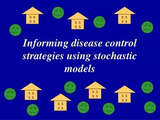
S S S S. S S S S. S S S S. S S S S. S S S S. S S S S. S S S S. Informing disease control strategies using stochastic models. Gastrointestinal Illness. # 2 cause of death in children worldwide Largely preventable Transmission pathways Contaminated water

E N D
S S S S S S S S S S S S S S S S S S S S S S S S S S S S Informing disease control strategies using stochastic models
Gastrointestinal Illness • # 2 cause of death in children worldwide • Largely preventable • Transmission pathways • Contaminated water • Lack of sanitation facilities • Poor hygiene
Question: • Suppose you are interested in reducing the burden of G.I. illness in children in a country that currently has a high burden of G.I. disease. • Also suppose that resources are limited • What intervention(s) should you implement? • Review recent literature
Previous Research • Fewtrell & Colford: meta-analyses of RCTs to reduce diarrhea, 2004 (Summary of results from developing countries) Intervention Studies Estimate 95%C.I. Hand Washing 5 0.56 (0.33, 0.93) Sanitation 2 0.68 (0.53, 0.87) Water Supply 4 1.03 (0.73, 1.46) Water Quality 15 0.69 (0.53, 0.89) Multiple 5 0.67 (0.59, 0.76)
What explains this variability? Effect estimates vary substantially from 0% reduction up to 85% reduction in G.I. illness ? ? ?
Some Considerations: • Randomization and blinding procedures (internal validity) • Generalizability (external validity) • Selection bias (participants are different than non-participants) • Publication bias (positive findings are more likely to be published)
Randomization and Blinding: • Randomization: ensures that comparison groups differ only by chance • Double blinding: ensures that neither the participant or investigator knows which treatment group the participant is in – prevents investigator/participant bias • Makes RCTs the gold standard of Epi studies
Randomization and Blinding: • Both are often missing in GI interventions • Fewtrell & Colford • 52 distinct studies • 16/52 (31%) employed randomization • 3/52 (3%) blinded participants to their exposure status
We Can Use Models • Statistical models? T h e d a t a a r e n o t r e a l l y i n d e p e n d e n t. Y I K E S ! W e n e e d a p a d d l e
Why Mathematical Models? • Controlled • Inexpensive • Able to handle complex interactions • Generate and test hypotheses • Provide explicit description of the system under study (as opposed to statistical models)
A note on models: • A primary goal of using models is not necessarily to come up with accurate predictions about the process under study, but is to observe and describe fundamental principles and relationships that emerge • Rule of thumb: don’t make it more complex than it needs to be!
Some model assumptions • Population is static: no one enters, no one leaves or dies • Individuals can only become infected once • People are equally likely to contact one another – there are no “networks” or cliques
2500 households 4 people per household All are initially susceptible S S S S S S S S S S S S S S S S S S S S S S S S S S S S Village Model
I S S S - People can become infected by being exposed to an infected person in their household - bh governs this route of infection
S S S S - People can become infected by being exposed to an infected person from another household in their community - bc governs this route of infection S I S S
S S S S • People can become infected by being exposed to • pathogens from the environment (does not include • drinking water) • - be governs this route of infection Pathogens from the Environment
S S S S • People can become infected by consuming pathogens • in drinking water • - bdw governs this route of infection Pathogens from drinking water
- Infected individuals shed pathogens into the drinking • water supply at a constant rate • - f governs the rate of shedding • The total number of pathogens shed is directly • dependent on the total number of infected individuals, Itotal f S I S I
S R S S • After time, infected people recover and are no longer • susceptible to infection • - r governs the time to recovery Household at time of Infection, T0 Household at time of Recovery, T1 r S I S S
Pathogens in drinking water and the environment • die off at a constant rate. • - m governs pathogen die off m Time = T1 Time = T2
Summary of routes of infection for any given individual Environment (not drinking water) be bc bh People from other households Household member Itotal * f bdw m Pathogens in source of drinking water Die off
Simulation steps • Determine hazards for each event • Determine time to next event • Determine type of event • Determine which household is affected • Update I, S, and R values for each household
Model Events • Five events can occur: • Infection via drinking water • Infection via a household member • Infection via another member of the village • Infection via the environment • Recovery • The number of Susceptibles (S), Infecteds (I), and Recovereds (R) for each household is updated after each event
Hazards • Hazards for each event are calculated based on transmission parameters, bc, bh, be, bdw, f, m, r And based on I and S • Hazards are calculated for each household, thus, each household has 5 hazards associated with it
Hazard Formulas • Hazard for infection via drinking water: ldw = bdw * Shh • Hazard for infection via household contact: lh = bh * Shh * Ihh • Hazard for infection via community contact: lc = bc * Shh * Itotal
Hazard Formulas • Hazard for infection via the environment: le = be * Shh • Hazard for recovery (moving from I to R): lr = r* Ihh
Time to Infection and Hazard • Recall that for an exponential distribution with mean = 1/l: P (T < t) = 1 – e-lt • This is a probability, it must be between 0 and 1
Time of Next Event • We know that 1-e-lt is between 0 and 1 • Solving for t: t = -log (1-p)/l • Thus, given a uniform random number and substituting it in for 1-p, we can randomly generate an event time that will come from an exponential distribution with mean = 1/l
Example • Suppose l = 2 • We generate 1000 random numbers between 0 and 1 and plug into the formula: t = -log (1-p)/2 • The resulting distribution of t looks like the following:
Time of Next Event • In our case the total hazard is the sum of all l’s, thus: lt = Sli • Time to next event is then: Tnext = - log (U(0,1)) / lt • The average time will be 1/lt
Which event occurred? Where? • We still need to determine which event will happen at Tnext and where it will happen ( which household) • Random numbers are employed to make these decisions
ldw1 lc1 lh1 lr1 le1 ldw2 le2 lc2 lh2 lr2 ldw3 Total l for Household #1 Total l for Household #2 • Remember that the total hazard is divided up into may smaller hazards for each event in each household
ldw1 lc1 lh1 lr1 le1 ldw2 le2 lc2 lh2 lr2 ldw3 Total l for Household #1 Total l for Household #2 • Randomly selecting a number between 0 and lt determines • which event happens and in which household • In the example below, an individual in household 2 is • infected from someone else in the community Random selection
Bookkeeping • After an event is determined, the appropriate household is updated so it has the correct number of I’s, S’s, and R’s • The process is then repeated: • New hazards are calculated • Tnext is determined • An event is selected • A household population is updated
When does it end? • After each time step the total time, T, is updated: T = T + Tnext • When T becomes greater than a predetermined value, the simulation stops.
So What? • Example questions this model can help to answer: • How do sanitation, hygiene, and water quality impact disease transmission? • Under what conditions is diarrheal disease endemic vs epidemic? • What amount of disease is attributable to drinking water?
How much disease is attributable to contaminated water? • Extremely difficult to answer this question with observational data or randomized controlled trials (experiments) • Bias due to confounding (observational data) • Bias due to lack of blinding and randomization procedures (RCT/experiments)
The ‘Perfect Study’ • We’d like to have two observations from everyone • Disease status with clean water • Disease status without clean water • In reality, we can only observe one outcome • Counterfactual outcomes are the hypothetical outcomes we don’t observe
An Example(?) Can’t observe both – but with models, WE CAN
Example: Water Quality Intervention • We run the model two times • First run: don’t allow people to become infected via drinking water. This is like “filtering” their water so that no exposure via drinking water is possible • Second run: normal run. We allow exposure via drinking water • In both runs we keep bh and bc relatively small
Example • Total cases with active filter = 412 • Total cases with placebo filter = 1651 • Total population = 10000 • Under these conditions (low bh, bc), (1651 – 412) / 1651 = .75 • 75 percent of cases could have been prevented if all drinking water would have been filtered
Example • Suppose we repeat this in a population where bh and bc are higher • Person-to-person transmission will be more of a factor
Example • Total cases with active filter = 5619 • Total cases with placebo filter = 7866 • Total population = 10000 • Under these conditions (high bh, bc), (7866 – 5619) / 7866 = .29 • 29 percent of cases could have been prevented if all drinking water would have been filtered
Impact • This example illustrates that the success of water quality interventions is dependent on the level of person-to-person (PTP) transmission occurring in a population • Water quality interventions will likely have more impact when PTP levels are low • They may not be the best choice in areas where PTP is high