Motion estimation

1. Motion estimation Digital Visual Effects Yung-Yu Chuang with slides by Michael Black and P. Anandan

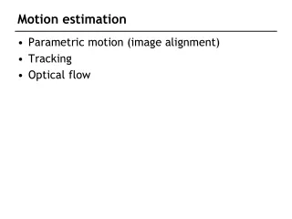
2. Motion estimation • Parametric motion (image alignment) • Tracking • Optical flow

3. Parametric motion direct method for image stitching

4. Tracking

5. Optical flow

6. Three assumptions • Brightness consistency • Spatial coherence • Temporal persistence

7. Brightness consistency Image measurement (e.g. brightness) in a small region remain the same although their location may change.

8. Spatial coherence • Neighboring points in the scene typically belong to the same surface and hence typically have similar motions. • Since they also project to nearby pixels in the image, we expect spatial coherence in image flow.

9. Temporal persistence The image motion of a surface patch changes gradually over time.

10. Image registration Goal: register a template image T(x) and an input image I(x), where x=(x,y)T. (warp I so that it matches T) Image alignment: I(x) and T(x) are two images Tracking: T(x) is a small patch around a point p in the image at t. I(x) is the image at time t+1. Optical flow: T(x) and I(x) are patches of images at t and t+1. warp I T fixed

11. Simple approach (for translation) • Minimize brightness difference

12. Simple SSD algorithm For each offset (u, v) compute E(u,v); Choose (u, v) which minimizes E(u,v); Problems: • Not efficient • No sub-pixel accuracy

13. Lucas-Kanade algorithm

14. Newton’s method • Root finding for f(x)=0 • March x and test signs • Determine Δx (small→slow; large→ miss)

15. Newton’s method • Root finding for f(x)=0

16. Newton’s method • Root finding for f(x)=0 Taylor’s expansion:

17. x0 Newton’s method • Root finding for f(x)=0 x2 x1

18. Newton’s method pick up x=x0 iterate compute update x by x+Δx until converge Finding root is useful for optimization because Minimize g(x) → find root for f(x)=g’(x)=0

19. Lucas-Kanade algorithm

20. Lucas-Kanade algorithm

21. Lucas-Kanade algorithm iterate shift I(x,y) with (u,v) compute gradient image Ix, Iy compute error image T(x,y)-I(x,y) compute Hessian matrix solve the linear system (u,v)=(u,v)+(∆u,∆v) until converge

22. Our goal is to find p to minimize E(p) translation affine Parametric model for all x in T’s domain

23. minimize Parametric model minimize with respect to

24. target image warped image image gradient Jacobian of the warp Parametric model

25. Jacobian matrix • The Jacobian matrix is the matrix of all first-order partial derivatives of a vector-valued function.

26. Jacobian matrix

27. target image warped image image gradient Jacobian of the warp Parametric model

28. Jacobian of the warp For example, for affine dxx dyx dxy dyy dx dy

29. Parametric model (Approximated) Hessian

30. Lucas-Kanade algorithm iterate • warp I with W(x;p) • compute error image T(x,y)-I(W(x,p)) • compute gradient image with W(x,p) • evaluate Jacobian at (x;p) • compute • compute Hessian • compute • solve • update p by p+ until converge

42. Coarse-to-fine strategy I J refine J Jw I warp + I J Jw pyramid construction pyramid construction refine warp + J I Jw refine warp +

43. Application of image alignment

44. Direct vs feature-based • Direct methods use all information and can be very accurate, but they depend on the fragile “brightness constancy” assumption. • Iterative approaches require initialization. • Not robust to illumination change and noise images. • In early days, direct method is better. • Feature based methods are now more robust and potentially faster. • Even better, it can recognize panorama without initialization.

45. Tracking

46. Tracking (u, v) I(x,y,t) I(x+u,y+v,t+1)

47. Tracking brightness constancy optical flow constraint equation

48. Optical flow constraint equation

49. Multiple constraints

50. Area-based method • Assume spatial smoothness