Understanding M-Channel Filter Banks: Structure, Applications, and Optimal Transform Derivation
460 likes | 579 Views
M-channel filter banks are essential in signal processing for effective analysis and synthesis. This document explores the fundamental principles of M-channel filter banks, detailing the relationship between input and output with and without decimators and interpolators. Additionally, it examines the conditions for perfect reconstruction and discusses the challenges of implementing FIR filters. Various applications in spectral analysis are presented, including the derivation of optimal transforms and the significance of decorrelation and energy compactness in efficient signal representation. A comprehensive understanding of aliasing errors and reconstruction techniques is also covered.

Understanding M-Channel Filter Banks: Structure, Applications, and Optimal Transform Derivation
E N D
Presentation Transcript
+ M-channel filter Bank vo(n) fo(n) o(n) yo(n) H0(z) G0(z) M M v1(n) f1(n) 1(n) y1(n) H1(z) G1(z) M M y(n) x(n) M-2(n) vM-2(n) fM-2(n) HM-2(z) GM-2(z) M M M-1(n) vM-1(n) fM-1(n) yM-1(n) HM-1(z) GM-1(z) M M Figure 31
M-channel filter Bank Without the decimator and interpolator, the input/output relationship is straightforward (32) With the decimator and interpolator, we have to take it step-by-step
M-channel filter Bank (33) (34) Decimated signal Images
M-channel filter Bank (33) (34) (35)
M-channel filter Bank (33) (34) (35) (36)
M-channel filter Bank (33) (34) (35) (36)
M-channel filter Bank (33) (34) (35) (36) (37)
M-channel filter Bank (33) (34) (35) (36) (37)
M-channel filter Bank (33) (34) (35) (36) (37)
M-channel filter Bank (38) Note Y(z) is a 1x1 matrix! (39) Alias Component (AC) matrix
M-channel filter Bank Aliasing error Aliasing error free condition (40)
M-channel filter Bank Aliasing error Aliasing error free condition (41)
M-channel filter Bank Condition for perfect reconstruction is simple in theory, as However, Is complicated to solve and resulted in IIR synthesis filters.
M-channel filter Bank An effective solution employing Polyphase decomposition Recalling, i.e., Or simply
M-channel filter Bank Similar treatment to the synthesis filter gives i.e., Or simply
M-channel filter Bank Diagram illustration: z-1 z-1 z-1
M-channel filter Bank Diagram illustration: z-1 z-1 z-1 Can be replaced with their polyphase components, as
M-channel filter Bank M M M M M M Can be replaced with their polyphase components, as
M-channel filter Bank M M z-1 z-1 M M z-1 z-1 z-1 z-1 M M
M M M M M M M-channel filter Bank z-1 z-1 z-1 z-1 z-1 z-1
M M M M M M M-channel filter Bank z-1 z-1 z-1 z-1 z-1 z-1 Results in perfect reconstruction
M-channel filter Bank Implementing FIR filters for M-channel filter banks, to begin with, Noted that
M-channel filter Bank Let Compute P(z)
M-channel filter Bank It can be seen that both analysis and synthesis filters are FIR
M-channel filter Bank All the analysis filters can be generated from
M-channel filter Bank All the analysis filters can be generated from
Spectral Analysis Given f(n) = [f0, f1, ..... , fN-1] and an orthonormal basis i.e., The spectral (generalized Fourier) coefficients of f(n) are defined as (66) (67) Eqn. 66 and 67 define the orthonormal transform and its inverse
Spectral Analysis If the members of are sinusoidal sequences, the transform is known as the Fourier Transform The Parseval theorem - Conservation of Energy in orthonormal transform (68)
An Application - Spectral Analysis 0 N N 1 f(n) N-1 N Figure 32 Orthonormal spectral analyser implemented with multirate filter bank
An Application - Spectral Analysis Transform efficiency - measured by decorrelation and energy compactness Correlation - Neighboring samples can be predicted from the current sample : an inefficient representation. Energy Compactness - The importance of each sample in forming the entire signal. If every sample is equally important, everyone of them has to be included in the representation: again an inefficient representation. An ideal transform: 1. Samples are totally unrelated to each other. 2. Only a few samples are necessary to represent the entire signal.
How to derive the optimal transform? Given a signal f(n), define the mean and autocorrelation as and (69) Assume f(n) is wide-sense stationary, i.e. its statistical properties are constant with changes in time Define and (70)
How to derive the optimal transform? (71) Equation 69 can be rewritten as (72) The covariance of f is given by (73)
How to derive the optimal transform? The signal is transform to its spectral coefficients with eqn 66 Comparing the two sequences:
How to derive the optimal transform? The signal is transform to its spectral coefficients with eqn 66 Comparing the two sequences: a. Adjacent terms are related b. Every term is important a. Adjacent terms are unrelated b. Only the first few terms are important
How to derive the optimal transform? The signal is transform to its spectral coefficients with eqn 66 similar to f, we can define the mean, autocorrelation and covariance matrix for
How to derive the optimal transform? a. Adjacent terms are related a. Adjacent terms are unrelated Adjacent terms are uncorrelated if every term is only correlated to itself, i.e., all off-diagonal terms in the autocorrelation function is zero. Define a measurement on correlation between samples: (74)
How to derive the optimal transform? We assume that the mean of the signal is zero. This can be achieved simply by subtracting the mean from f if it is non-zero. The covariance and autocorrelation matrices are the same after the mean is removed.
How to derive the optimal transform? b. Only the first few terms are important b. Every term is important Note: If only the first L-1 terms are used to reconstruct the signal, we have (75)
How to derive the optimal transform? If only the first L-1 terms are used to reconstruct the signal, the error is (76) The energy lost is given by (77) but, (78) hence
How to derive the optimal transform? Eqn. 78 is valid for describing the approximation error of a single sequence of signal data f. A more generic description for covering a collection of signal sequences is given by: (79) An optimal transform mininize the error term in eqn. 79. However, the solution space is enormous and constraint is required. Noted that the basis functions are orthonormal, hence the following objective function is adopted.
How to derive the optimal transform? (80) The term r is known as the Lagrangian multiplier The optimal solution can be found by setting the gradient of J to 0 for each value of r, i.e., (81) Eqn 81 is based on the orthonormal property of the basis functions.
How to derive the optimal transform? The solution for each basis function is given by (82) ris an eigenvector of Rf and r is an eigenvalue Grouping the N basis functions gives an overall equation (83) R= Rf= which is a diagonal matrix. The decorrelation criteria is satisfied (84)
![[0 1 0]](https://cdn0.slideserve.com/536424/slide1-dt.jpg)