Download
1 / 45
450 likes | 470 Views
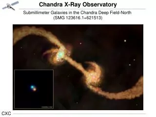
AGN deep multiwavelength surveys: the case of the Chandra Deep Field South. Fabrizio Fiore Simonetta Puccetti, Giorgio Lanzuisi. Table of content. Introduction Big scenario for structure formation: AGN & galaxy co-evolution SMBH census: search for highly obscured AGN X-ray surveys

E N D
AGN deep multiwavelength surveys:the case of the Chandra Deep Field South Fabrizio Fiore Simonetta Puccetti, Giorgio Lanzuisi
Table of content • Introduction • Big scenario for structure formation: AGN & galaxy co-evolution • SMBH census: search for highly obscured AGN • X-ray surveys • Unobscured and moderately obscured AGN density • Infrared surveys • Compton thick AGN • CDFS 2Msec observation: the X-ray view of IR bright AGN: • Spectra of IR sources directly detected in X-rays • X-ray “stacking” analysis of the sources not directly detected.
Two seminal results: • The discovery of SMBH in the most local bulges; tight correlationbetween MBH and bulge properties. • The BH mass density obtained integrating the AGN L.-F. and the CXB ~ that obtained from local bulges Co-evolution of galaxies and SMBH most BH mass accreted during luminous AGN phases! Most bulges passed a phase of activity: • Complete SMBH census, • 2) full understanding of AGN feedback • are key ingredients to understand galaxy evolution
To prove this scenario we need to have: • Complete SMBH census, • Physical models for AGN feedbacks • Observational constraints to these models AGN and galaxy co-evolution • Early on • Strong galaxy interactions= violent star-bursts • Heavily obscured QSOs • When galaxies coalesce • accretion peaks • QSO becomes optically visible as AGN winds blow out gas. • Later times • SF & accretion quenched • red spheroid, passive evolution
Evidences for missing SMBH While the CXB energy density provides a statistical estimate of SMBH growth, the lack, so far, of focusing instrument above 10 keV (where the CXB energy density peaks), frustrates our effort to obtain acomprehensive picture of the SMBH evolutionary properties. Gilli et al. 2007 43-44 44-44.5 Marconi 2004-2007 Menci , Fiore et al. 2004, 2006, 2008
42-43 43-44 44-44.5 44.5-45.5 >45.5 AGN density La Franca, Fiore et al. 2005 Menci, Fiore et al. 2008 Paucity of Seyfert like sources @ z>1 is real? Or, is it, at least partly, a selection effect? Are we missing in Chandra and XMM surveys highly obscured (NH1024 cm-2) AGN? Which are common in the local Universe…
Highly obscured Mildly Compton thick INTEGRAL survey ~ 100 AGN Sazonov et al. 2006
Central engine Dusty torus Completing the census of SMBH • X-ray surveys: • very efficient in selecting unobscured and moderately obscured AGN • Highly obscured AGN recovered only in ultra-deep exposures • IR surveys: • AGNs highly obscured at optical and X-ray wavelengths shine in the MIR thanks to the reprocessing of the nuclear radiation by dust
X-ray-MIR surveys • CDFS-Goods MUSIC catalog(Grazian et al. 2006, Brusa, FF et al. 2008) Area 0.04 deg2 • ~200 X-ray sources, 2-10 keV down to 210-16 cgs, 0.5-2 keV down to 510-17 cgs 150 spectroscopic redshifts • 1100 MIPS sources down to 40 Jy, 3.6m detection down to 0.08 Jy • Ultradeep Optical/NIR photometry, R~27.5, K~24 • ELAIS-S1 SWIRE/XMM/Chandra survey(Puccetti, FF et al. 2006, Feruglio,FF et al. 2007, La Franca, FF et al. 2008). Area 0.5 deg2 • 500 XMM sources, 205 2-10 keV down to 310-15 cgs, >half with spectroscopic redshifts. • 2600 MIPS sources down to 100 Jy, 3.6m detection down to 6 Jy • Relatively deep Optical/NIR photometry, R~25, K~19 • COSMOSXMM/Chandra/Spitzer. Area ~1 deg2 • ~1700 Chandra sources down to 610-16 cgs, >half with spectroscopic redshifts. • 900 MIPS sources down to 500 Jy, 3.6m detection down to 10 Jy, R~26.5 • In future we will add: • CDFS-Goods, Chandra 2Msec observation • CDFN-Goods • COSMOS deep MIPS survey
z = 0.73 structure 40 arcmin 52 arcmin z-COSMOS faint Full COSMOS field Color: XMM first year Chandra deep and wide fields CDFS 2Msec 0.05deg2 CCOSMOS 200ksec 0.5deg2 100ksec 0.4deg2 ~400 sources 1.8 Msec ~1800 sources Elvis et al. 2008 20 arcmin 1 deg
AGN directly detected in X-rays Open circles=logNH>23 Open squares = MIR/O>1000 sources (Tozzi et al. 2003)
MIR selection of CT AGN Fiore et al. 2003 ELAIS-S1 obs. AGN ELAIS-S1 24mm galaxies HELLAS2XMM CDFS obs. AGN Unobscured obscured MIR/O Open symbols = unobscured AGN Filled symbols = optically obscured AGN X/0
MIR selection of CT AGN Fiore et al. 2008a Fiore et al. 2008b CDFS X-ray HELLAS2XMM GOODS 24um galaxies COSMOS X-ray COSMOS 24um galaxies R-K Open symbols = unobscured AGN Filled symbols = optically obscured AGN * = photo-z
GOODS MIR AGNs F24/FR>1000 R-K>4.5 • <SFR-IR>~200!! Msun/yr • <SFR-UV>~7!! Msun/yr • <SFR-X>~65 Msun/yr F24um/FR<200 R-K>4.5 • <SFR-IR> ~ 18 Msun/yr • <SFR-UV> ~13 Msun/yr • <SFR-X>~20 Msun/yr Stack of Chandra images of MIR sources not directly detected in X-rays • F24um/FR>1000 R-K>4.5 • logF(1.5-4keV) stacked sources=-17 @z~2 logLobs(2-8keV) stacked sources ~41.8 • log<LIR>~44.8==> logL(2-8keV) unabs.~43 • Difference implieslogNH~24 Fiore et. al. 2008a
Program of the project (1) • Selection of IR sources with X-ray detection which are likely to host a highly obscured AGN • Extraction of the Chandra spectra of these sources from the event files • Characterization of the X-ray spectra: estimate of the absorbing column density • Evaluation of systematic errors: • Background evaluation • Combination of data from different observations
Program of project (2) • Selection of IR sources without a direct X-ray detection which are likely to host a highly obscured AGN • ‘Stacking’ of X-ray images at the position of these sources • Analysis of the ‘stacked’ images
X-ray (and multiwavelength) surveys Fabrizio Fiore
Table of content • A historical perspective • Tools for the interpretation of survey data • Number counts • Luminosity functions • Main current X-ray surveys • What next
A historical perspective • First survey of cosmological objects: radio galaxies and radio loud AGN • The discovery of the Cosmic X-ray Background • The first imaging of the sources making the CXB • The resolution of the CXB • What next?
Radio sources number counts First results from Cambridge surveys during the 50’: Ryle Number counts steeper than expected from Euclidean universe
Number counts Flux limited sample: all sources in a given region of the sky with flux > than some detection limit Flim. • Consider a population of objects with the same L • Assume Euclidean space
Number counts Test of evolution of a source population (e.g. radio sources). Distances of individual sources are not required, just fluxes or magnitudes: the number of objects increases by a factor of 100.6=4 with each magnitude. So, for a constant space density, 80% of the sample will be within 1 mag from the survey detection limit. If the sources have some distribution in L:
Problems with the derivation of the number counts • Completeness of the samples. • Eddington bias: random error on mag measurements can alter the number counts. Since the logN-logFlim are steep, there are more sources at faint fluxes, so random errors tend to increase the differential number counts. If the tipical error is of 0.3 mag near the flux limit, than the correction is 15%. • Variability. • Internal absorption affects “color” selection. • SED, ‘K-correction’, redshift dependence of the flux (magnitude).
Optically selected AGN number counts z<2.2 B=22.5 100 deg-2 B=19.5 10 deg-2 z>2.2 B=22.5 50 deg-2 B=19.5 1 deg-2 B-R=0.5
X-ray AGN number counts <X/O> OUV sel. AGN=0.3 R=22 ==> 310-15 1000deg-2 R=19 ==> 510-14 25deg-2 The surface density of X-ray selected AGN is 2-10 times higher than OUV selected AGN
The Cosmic X-ray Background Giacconi (and collaborators) program: 1962 sounding rocket 1970 Uhuru 1978 HEAO1 1978 Einstein 1999 Chandra!
The Cosmic X-ray Background • The CXB energy density: • Collimated instruments: • 1978 HEAO1 • 2006 BeppoSAX PDS • 2006 Integral • 2008 Swift BAT • Focusing instruments: • 1980 Einstein 0.3-3.5 keV • 1990 Rosat 0.5-2 keV • 1996 ASCA 2-10 keV • 1998 BeppoSAX 2-10 keV • 2000 RXTE 3-20 keV • 2002 XMM 0.5-10 keV • 2002 Chandra 0.5-10 keV • 2012 NuSTAR 6-100 keV • 2014 Simbol-X 1-100 keV • 2014 NeXT 1-100 keV • 2012 eROSITA 0.5-10 keV • 2020 IXO 0.5-40 keV
The V/Vmax test Marteen Schmidt (1968) developed a testfor evolution not sensitive to the completeness of the sample. Suppose we detect a source of luminosity L and flux F >Flim at a distance rin Euclidean space: If we consider a sample of sources distributed uniformly, we expect that half will be found in the inner half of the volume Vmax and half in the outer half. So, on average, we expect V/Vmax=0.5
The V/Vmax test In an expanding Universe the luminosity distance must be used in place of r and rmax and the constant density assumption becomes one of constant density per unit comuving volume .
Luminosity function In most samples of AGN <V/Vmax> > 0.5. This means that the luminosity function cannot be computed from a sample of AGN regardless of their z. Rather we need to consider restricted z bins. More often sources are drawn from flux-limited samples, and the volume surveyed is a function of the Luminosity L. Therefore, we need to account for the fact that more luminous objects can be detected at larger distances and are thus over-represented in flux limited samples. This is done by weighting each source by the reciprocal of the volume over which it could have been found:
Assume that the intrinsic spectrum of the sources making the CXB has E=1 I0=9.810-8 erg/cm2/s/sr ’=4I0/c
Optical (and soft X-ray) surveys gives values 2-3 times lower than those obtained from the CXB (and of the F.&M. and G. et al. estimates)
CDFN-CDFS 0.1deg2 Barger et al. 2003; Szokoly et al. 2004 -16 E-CDFS 0.3deg2 Lehmer et al. 2005 EGS/AEGIS 0.5deg2 Nandra et al. 2006 C-COSMOS 0.9 deg2 -15 Flux 0.5-10 keV (cgs) ELAIS-S1 0.5 deg2 Puccetti et al. 2006 XMM-COSMOS 2 deg2 HELLAS2XMM 1.4 deg2 Cocchia et al. 2006 Champ 1.5deg2 Silverman et al. 2005 -14 SEXSI 2 deg2 Eckart et al. 2006 -13 XBOOTES 9 deg2 Murray et al. 2005, Brand et al. 2005 Pizza Plot Area A survey of X-ray surveys
A survey of X-ray surveys Point sources Clusters of galaxies
A survey of surveys Main areas with large multiwavelength coverage: • CDFS-GOODS 0.05 deg2: HST, Chandra, XMM, Spitzer, ESO, Herschel, ALMA • CDFN-GOODS 0.05 deg2: HST, Chandra, VLA, Spitzer, Hawaii, Herschel • AEGIS(GS) 0.5 deg2: HST, Chandra, Spitzer, VLA, Hawaii, Herschel • COSMOS 2 deg2: HST, Chandra, XMM, Spitzer, VLA, ESO, Hawaii, LBT, Herschel, ALMA • NOAO DWFS 9 deg2 : Chandra, Spitzer, MMT, Hawaii, LBT • SWIRE 50 deg2(Lockman hole, ELAIS, XMMLSS,ECDFS): Spitzer, some Chandra/XMM, some HST, Herschel • eROSITA! 20.000 deg2 10-14 cgs 200 deg2 310-15 cgs
z = 0.73 structure 40 arcmin 52 arcmin z-COSMOS faint Full COSMOS field Color: XMM first year Chandra deep and wide fields CDFS 2Msec 0.05deg2 CCOSMOS 200ksec 0.5deg2 100ksec 0.4deg2 ~400 sources 1.8 Msec ~1800 sources Elvis et al. 2008 20 arcmin 1 deg
XMM surveys COSMOS 1.4Msec 2deg2 Lockman Hole 0.7Msec 0.3deg2
Chandra surveys AEGIS: Extended Groth Strip Bootes field
Elais-N1 Elais-S1 Elais-N2 LockmanHole XMM-LSS Spitzer large area surveys: SWIRE
eROSITA ~30ks on poles, ~1.7ksec equatorial
log Energy range 1 10 100 keV -13 -15 -17 cgs log Sensitivity Log Area deg2 4 2 0 What next? The X-ray survey discovery space NS NeXT SX IXO ASCA/BSAX XMM ChandraIXO Einstein ROSAT BSAX/ASCA XMM Swift ROSAT eROSITA