Download

1 / 17
170 likes | 292 Views
Non-equilibrium materials – maximum strength under extreme conditions. Alfred Hübler Center for Complex Systems Research University of Illinois at Urbana-Champaign. Research supported in part by the National Science Foundation ( DMS-03725939 ITR ). We study:

E N D
Non-equilibrium materials – maximum strength under extreme conditions Alfred Hübler Center for Complex Systems Research University of Illinois at Urbana-Champaign Research supported in part by the National Science Foundation (DMS-03725939 ITR)
We study: • The strength of materials with large heat flow • Typical structure of materials with a large flow: Structure of materials with high-voltage currents • We find: • Materials have their maximum strength in a large heat flow if they are produced in a large heat flow. • -Materials produced in a high-voltage current develop fractal structures which maximize the conductivity for the applied current. These fractal structures can be predicted with graph-theoretical models.
Strength of materials with large heat flow ↓heat flow α = Linear expansion coefficient:, c1=Tensile stiffness, c2 = Nonlinear stiffness, k=conductivity Production temperatures: T1,p, T2,p <=> heat flow Qp= k (T1,p- T2,p) Application temperatures: T1, T2 <=> heat flow Q= k (T1- T2) Equilibrium length at production temperatures: xp = x1,0 (1+ α T1,p) = x2,0 (1+ α T2,p) Equilibrium lengths at application temperatures: x1 = x1,0 (1+ α T1), x2 = x2,0 (1+ α T2) Tensile stresses: F1 = c1 (x-x1)-c2 (x-x1)2 , if x-x1 < c1/(2c2) F2 = c1 (x-x2) -c2 (x-x2)2, if x-x2 < c1/(2c2)
Strength of materials with a large heat flow Net tensile stress: Fn(x) =F1(x)+F2(x) Strength: F = max(Fn(x)) Stength F depends on production temperatures and application temperatures. Result: The material has maximum application strength if the production temperatures match the application temperatures, i.e. Production heat flow Qp = Application heat flow Q Figure 1. The strength versus the production temperature T2,p , where T1,p=10. The application temperatures are T1=10, and T2=20, for α=1, c1=0.95, c2=1
Experimental Study of Structural Changes in Materials due to High-voltage Currents:Growth of Fractal Transportation Networks needle electrode sprays charge over oil surface 20 kV air gap between needle electrode and oil surface approx. 5 cm ring electrode forms boundary of dish has a radius of 12 cm oil height is approximately 3 mm, enough to cover the particles castor oil is used: high viscosity, low ohmic heating, biodegradable particles are non-magnetic stainless steel, diameter D=1.6 mm particles sit on the bottom of the dish
Phenomenology Overview { 12 cm stage I: strand formation t=0s 10s 5m 13s 14m 7s { 14m 14s 14m 41s 15m 28s 77m 27s stage II: boundary connection stage III: geometric expansion stationary state
Adjacency defines topological species of each particle Termini = particles touching only one other particle Branching points = particles touching three or more other particles Trunks = particles touching only two other particles Particles become termini or three-fold branch points in stage III. In addition there are a few loners (less than 1%). Loners are not connected to any other particle. There are no closed loops in stage III.
Relative number of each species is robust Graphs show how the number of termini, T, and branching points, B, scale with the total number of particles in the tree.
Qualitative effects of initial distribution N = 752 T = 149 B = 146 N = 785 T = 200 B = 187 N = 720 T = 122 B = 106 N = 752 T = 131 B = 85 (N = Number of Particles, T = Number of Termini, B=Number of Branch Points)
? Can we predict the structure of the emerging transportation network?
Predicting the Fractal Transporatation Network Left: Initial condition, Right: Emergent transporation network
Predictions of structural changes in materials due to a high voltage current: Predicting fractal network growth loner Task: Digitize stage II structure and predict stage III transporation network. 1) Determine neighbors, since particles can only connect to their neighbors. All the links shown on the left are potential connections for the final tree. 2) Use a graph-theoretical algorithms to connect particles, until all available particles connect into a tree. Some particles will not connect to any others (loners). They commonly appear in experiments. We test three growth algorithms: 1) Random Growth: Randomly select two neighboring particles & connect them, unless a closed loop is formed(RAN) 2) Minimum Spanning Tree Model: Randomly select pair of very close neighbors & connect them, unless a closed loop is formed(MST) 3) Propagating Front Model: Randomly select pair of neighbors, where one of them is already connected & connect them, unless a closed loop is formed(PFM)
Random Growth Model: Randomly select two neighboring particles Typical connection structure from RAN algorithm. Distribution of termini produced from 105 permutations run on a single experiment. Number of termini produced for all experiments, plotted as a function of N.
Minimum Spanning Tree Model: Randomly select pair of very close neighbors Typical connection structure from MST algorithm. Distribution of termini produced from 105 permutations run on a single experiment. Number of termini produced for all experiments, plotted as a function of N.
Propagation Front Model: Randomly select connected pair of neighbors Typical connection structure from PFM algorithm. Distribution of termini produced from 105 permutations run on a single experiment. Number of termini produced for all experiments, plotted as a function of N.
Comparison of all models to experiments Main Result: The Minimum Spanning Tree (MST) growth model is the best predictor of the emerging fractal transportation network
Structural changes of materials in high voltage current random initial distribution compact initial distribution • Experiment:J. Jun, A. Hubler, PNAS 102, 536 (2005) • Three growth stages: strand formation, boundary connection, and geometric expansion; • Networks are open loop; • Statistically robust features: number of termini, number of branch points, resistance, initial condition matters somewhat; • 4) Minimum spanning tree growth model predicts emerging pattern. • 5) To do: random initial condition, predict other observables, control network growth, study fractal structures in systems with a large heat flow • Applications: Hardware implementation of neural nets, absorbers, batteries • M. Sperl, A Chang, N. Weber, A. Hubler, Hebbian Learning in the Agglomeration of Conducting Particles, Phys.Rev.E. 59, 3165 (1999) • Come to Physics 510!