Download

1 / 44
440 likes | 538 Views
Delve into the rich history of system identification and encounter various obstacles faced in nonlinear system identification. Explore effective solutions, computation methods, and the application of the Sequential Importance Resampling technique. Discover the Expectation-Maximisation algorithm and its significance in estimating complex systems.

E N D
Some System Identification Challenges and Approaches “Many basic scientific problems are now routinely solved by simulation: a fancy random walk is performed on the system of interest. Averages computed from the walk give useful answers to formerly intractable problems” Persi Diaconis, 2008 • Brett Ninness • School of Electrical Engineering & Computer Science • The University of Newcastle, Australia
System Identification - a rich history • 1700‘s: Bernoulli, Euler, Lagrange - probability concepts • 1763:Bayes- conditional probability • 1795:Gauss, Legendre - least squares • 1800-1850:Gauss, Legendre, Cauchy - prob. distributions • 1879:Stokes - periodogram of time series • 1890:Galton, Pearson - regression and correlation • 1922:Fisher - Maximum Likelihood (ML) • 1921:Yule - AR and MA time series • 1933:Kolmogorov - Axiomatic probability theory • 1930‘s:Khinchin, Kolmogorov, Cramér - stationary processes
System Identification - a rich history • 1941-1949: Wiener, Kolmogorov - prediction theory • 1960:Kalman - Kalman Filter • 1965:Kalman & Ho - Realisation theory • 1965:Åström & Bohlin - ML methods for dynamic systems • 1970:Box & Jenkins - a unified and complete presentation • 1970’s: Experiment design, PE formulation with underpinning theory, analysis of recursive methods • 1980‘s: Bias & Variance quantification, tradeoff and design • 1990‘s: Subspace methods, control relevant identification, robust estimation methods.
Acknowledgements • Results here rest heavily on the work of colleagues: • Dr. Adrian Wills (Newcastle University) • Dr. Thomas Schön (Linköping University) • Dr. Stuart Gibson (Nomura Bank) • Soren Henriksen (Newcastle University) • and on learning from experts: • Håkan Hjalmarsson, Tomas McKelvey, Fredrik Gustafsson, Michel Gevers, Graham Goodwin.
Challenge 1 - General Nonlinear ID • Effective solutions available for specific nonlinear structures • NARX, Hammerstein-Wiener, Bilinear..... • Extension to more general forms? • Example:
Challenge 1 - General Nonlinear ID Obstacle 1: How do we compute a cost function? • Prediction error (PE) cost: • Maximum Likelihood (ML) cost:
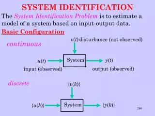
Computing • Turn to general measurement and time update equations: Measurement Update Time Update • Problem - closed form solutions only for special cases: • Linear, Gaussian (Kalman Filter), Discrete state HMM • More generally: • Need to compute solution numerically • Multi-dimensional integrals the main challenge
SEQUENTIAL IMPORTANCE RESAMPLING • SIR - More commonly known as “particle filtering” • Key idea - use the strong law of large numbers (SLLN) • Suppose a vector random number generator gives realisations from a given target density • Then by the SLLN, with probability one: • Suggests approximate quantification • How to build the necessary random number generator?
Recursive solution (Particle filter) Time Update Resampling Measurement Update
Example vs.
History • Handschin & Mayne, Int’l J. Control, 1969 • Resampling Approach: Gordon, Salmond & Smith, IEE Proc. Radar & Signal Processing, 1993. (1136 citations) • Now widely used in signal processing, target tracking, computer vision, econometrics, robotics and statistics, control.... • Some applications in system identification. • Bulk of work has involved considering parameters as state variables.
Back to Nonlinear System Identification • General(ish) model structure • Prediction error cost: • Max. Likelihood cost:
Nonlinear System Identification Obstacle 2: How do we compute an estimate? • Gradient based search is standard practice: • How to compute the necessary gradients? • Strategies: • Differencing to compute derivatives? • Direct search methods: Nelder-Mead, simulated annealing?
Expectation-Maximisation (EM) ALG. • Example - linear system: • Estimate by regression? • Need state - use estimate? E.g. Kalman smoother • Suggests iteration: • Use estimates of A,B,C,D to estimate state ; • Use estimates of state to estimate A,B,C,D; • Return and do again.
Expectation-Maximisation (EM) ALG. • Key idea - “complete” and “incomplete” data • Actual observations: • “Wished for” (incomplete) obervations: • Form estimate of “wished for” likelihood: • E Step: Calculate • M Step: Compute
KEY EM Algorithm Property • Bayes’ rule: • Take conditional expectation of both sides: • Increasing implies increased likelihood:
Expectation-Maximisation (EM) ALG. • History • Generally attributed to Baum: Ann. Math. Stat. 1970; • Generalised by Dempster et al: JRSS B, 1977 (9858 cites) • Widely used in image processing, statistics, radar...
Nonlinear system estimation Example: N=100 data points, M=100 particles, 100 experiments
Evolution of • Look at b parameter only - others fixed at true values:
Gradient Based Search Revisited • Fisher’s Identity
Challenge 2: Application Relevant ID • “Traditional” practice - note asymptotic results • Quality of an estimate must be quantified for it to be useful • Assume convergence effectively occurred for finite N
Assessment & Design • Often, a function of the parameters is of more interest • Again - “classical” approach - use linear approximation: • Couple with approximate Gaussianity of
One perspective Need to combine prior knowledge, assumptions and data : Measure of the evidence supporting an underlying system property - parameter value, frequency response, achieved gain/phase margin......
Computing Posteriors • In principle, posterior computation straightforward: Bayes’ Rule Likelihood prior knowledge • Example: Combine:
Using Posteriors Now the difficulty - using the posterior • Marginal on i’th parameter: • Evaluation on -dim. grid, evaluations of • Simpson’s rule - evaluation error: model order • Other measures?
A randomised approach • Use the Strong Law of Large Numbers (SLLN) again. • Build a (vector) random number generator giving realisations: • Then by the SLLN, with probability one: • Suggests the approximation: • One view - numerical integration with intelligently chosen grid points.
The Metropolis Algorithm The required vector random number generator: • 1. Initialise: Choose and set Z.y=y; Z.u=u; M.A=4; g1=est(Z,M); theta=g1.theta;
The Metropolis Algorithm • 2. Draw a proposal value xi = theta + 0.1*randn(size(theta)); g2 = theta2m(xi,g1);
The Metropolis Algorithm 3. Compute an acceptance probability: cold = validate(Z,g1); cnew = validate(Z,g2); prat = exp((-0.5/var)*(cold-cnew)*N); alpha = min(1,prat);
The Metropolis Algorithm 4. Set with probability if (rand <= alpha) theta=xi; end;
“Markov Chain Monte Carlo” History • Origins: Metropolis, Rosenbluth, Rosenbluth,Teller & Teller, Journal of Chemical Physics, 1953. (11,564 ISI citations) • Widespread use: • Listed #1 in “Great Algorithms of Scientific Computing”, Dongarra & Sullivan, Comp. & Sci in Eng. 2000 • “The Markov Chain Monte Carlo Revolution”, Diaconis, Bull. American Mathematical Society, 2008. “Many basic scientific problems are now routinely solved by simulation: a fancy random walk is performed on the system of interest. Averages computed from the walk give useful answers to formerly intractable problems” • Widely used in chemistry, physics, statistics.... Emerging uses in biology, telecommunications.
Example • Simple first order situation: • N=20 data samples available: • Metropolis Algorithm: realisations
Posterior of functions of • Candidate closed loop controller: What are the likely achieved gain and phase margins ? Implicit functions of - direct computation unclear
Sample Histograms of There is strong evidence that the proposed controller will achieve a gain margin > 3.8 and phase margin > 95o
Conclusions • Many thanks for your attention; • Collective thanks to the SYSID2009 Organisation Team! • Deep thanks to the Uni. Newcastle Signal Processing Micro-electonics group (sigpromu.org) • Steve Weller, Chris Kellett, TharakaDissanayake, Peter Schreier, Sarah Johnson, Geoff Knagge, BjörnRüffer, Adrian Wills, Lawrence Ong, Dale Bates, Ian Griffiths, David Hayes, SorenHenriksen, Adam Mills, Alan Murray who endured multiple road-test versions of this talk, that were even worse than this one.