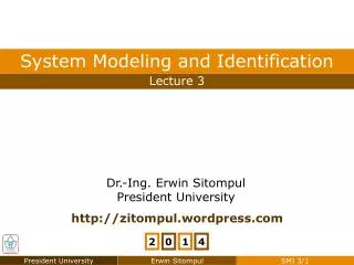
Solution to Homework 1
Chapter 2. Examples of Dynamic Mathematical Models. Solution to Homework 1. q i. A 1 : Cross-sectional area of the first tank [m 2 ] A 2 : Cross-sectional area of the second tank [m 2 ] h 1 : Height of liquid in the first tank [m]

Solution to Homework 1
E N D
Presentation Transcript
Chapter 2 Examples of Dynamic Mathematical Models Solution to Homework 1 qi A1 : Cross-sectional area of the first tank [m2] A2 : Cross-sectional area of the second tank [m2] h1 : Height of liquid in the first tank [m] h2 : Height of liquid in the second tank [m] h1 h2 q1 qo a1 a2 v2 v1 • The process variable are now the heights of liquid in both tanks, h1 and h2. • The mass balance equation for this process yields:
Chapter 2 Examples of Dynamic Mathematical Models Solution to Homework 1 • Assuming ρ, A1, and A2 to be constant, we obtain: • After substitution and rearrangement,
Chapter 2 Examples of Dynamic Mathematical Models Homework 2 Build a Matlab-Simulink model for the interacting tank-in-series system and perform a simulation for 200 seconds. Submit the mdl-file (softcopy) and the screenshots of the Matlab-Simulink file and the scope of h1 and h2 as the homework result (hardcopy). Use the following values for the simulation. a1 = 210–3 m2 a2 = 210–3 m2 A1 = 0.25 m2 A2 = 0.10 m2 g = 9.8 m/s2 qi = 510–3m3/s tsim = 200 s
Chapter 2 Examples of Dynamic Mathematical Models Homework 2 (New) Build a Matlab-Simulink model for the triangular-prism-shaped tank and perform a simulation for 200 seconds. Submit the mdl-file (softcopy) and the screenshots of the Matlab-Simulink file and the scope of h as the homework result (hardcopy). Use the following values for the simulation. NEW a= 210–3 m2 Amax= 0.5 m2 hmax = 0.7 m h0 = 0.05 m (!) g = 9.8 m/s2 qi1 = 510–3 m3/s qi2 = 110–3 m3/s tsim = 200 s
Chapter 2 Examples of Dynamic Mathematical Models Heat Exchanger • Consider a heat exchanger for the heating of liquids as shown below. Assumptions: • Heat capacity of the tank is small compare to the heat capacity of the liquid. • Spatially constant temperature inside the tank as it is ideally mixed. • Constant incoming liquid flow, constant specific density, and constant specific heat capacity.
Chapter 2 Examples of Dynamic Mathematical Models Heat Exchanger • Consider a heat exchanger for the heating of liquids as shown below. Tl q Tl : Temperature of liquid at inlet [K] Tj : Temperature of jacket [K] T : Temperature of liquid inside and at outlet [K] q : Liquid volume flow rate [m3/s] V : Volume of liquid inside the tank [m3] ρ : Liquid specific density [kg/m3] cp : Liquid specific heat capacity [J/(kgK)] V ρ T cp T q Tj
Chapter 2 Examples of Dynamic Mathematical Models Heat Exchanger • The heat balance equation becomes: A : Heat transfer area of the wall [m2] a : Heat transfer coefficient [W/(m2K)] • Rearranging: • The heat exchanger will be in steady-state if dT/dt = 0, so the steady-state temperature at outlet is:
Chapter 2 Examples of Dynamic Mathematical Models Series of Heat Exchangers • Consider a series of heat exchangers where a liquid is heated. T0 T1 T2 Tn–1 Tn V1 T1 V2 T2 Vn Tn w1 w2 w3 Assumptions: • Heat flows from heat sources into liquid are independent from liquid temperature. • Ideal liquid mixing and zero heat losses. • Accumulation ability of exchangers walls is neglected • Flow rates and liquid specific heat capacity are constant
Chapter 2 Examples of Dynamic Mathematical Models Series of Heat Exchangers • Under these circumstances, the following heat balances result: t : Time variable [s] T0 : Liquid temperature in the first tank inlet [K] Ti : Liquid temperature inside the i-th heat exchanger [K] Vi : Liquid temperature inside the i-th heat exchanger [m3] q : Volume flow rate [m3/s] ρ: Liquid density [kg/m3] wi : Heat inputs [W] • The process input variables are heat inputs wiand the first tank inlet temperature T0. • The process state variables are temperatures T1, ... Tn. • Initial conditions, i.e., initial temperatures in heat exchangers, are arbitrary. T1(0) = T10, ..., Tn(0) = Tn0. • The output variables can be chosen up to the interest of the user.
Chapter 2 Examples of Dynamic Mathematical Models Series of Heat Exchangers • The series of heat exchangers will be in a steady-state if: • Let the steady-state values of the process inputs wi, T0 be given, the steady-state temperatures inside the exchangers are:
Chapter 2 Examples of Dynamic Mathematical Models Double-Pipe Heat Exchanger • A single-pass, double-pipe steam heat exchanger is shown below. The liquid in the inner tube is heated by condensing steam. τ : Space variable [m] Ti : Liquid temperature in the inner tube [K] Ti(τ,t) To : Liquid temperature in the outer tube [K] To(t) q : Liquid volume flow rate in the inner tube[m3/s] ρ : Liquid specific density in the inner tube [kg/m3] cp : Liquid specific heat capacity [J/(kgK)] A : Heat transfer area per unit length [m] Ai : Cross-sectional area of the inner tube [m2] q τ To,ss Ti,ss τ dτ L • Heat transfer modes: convection (through the moving fluid) and conduction (across the metal of the inner tube
Chapter 2 Examples of Dynamic Mathematical Models Double-Pipe Heat Exchanger • The profile of temperature Ti of an element of heat exchanger with length dτ for time dt is given by: To(t) Ti(τ,t) (taken as approximation) dτ • The heat balance equation of the element can be derived as:
Chapter 2 Examples of Dynamic Mathematical Models Double-Pipe Heat Exchanger • The equation can be rearrange to give: • The boundary condition is Ti(0,t) and Ti(L,t). • The initial condition is Ti(τ,0).
Chapter 2 Examples of Dynamic Mathematical Models Heat Conduction in a Solid Body • Consider a metal rod of length L with ideal insulation. • Heat is brought in on the left side and withdrawn on the right side. • Changes of heat flows q(0) and q(L) influence the rod temperature T(x,t). • The heat conduction coefficient, density, and specific heat capacity of the rod are assumed to be constant. q(0) q(L) q(x) q(x+dx) x dx L
Chapter 2 Examples of Dynamic Mathematical Models Heat Conduction in a Solid Body q(0) q(L) q(x) q(x+dx) dx x L t : Time variable [s] x : Space variable [m] T : Rod temperature [K] T(x,t) ρ : Rod specific density [kg/m3] A : Cross-sectional area of the rod [m2] cp : Rod specific heat capacity [J/(kgK)] q(x): Heat flow density at length x [W/m2] q(x+dx) : Heat flow density at length x+dx [W/m2]
Chapter 2 Examples of Dynamic Mathematical Models Heat Conduction in a Solid Body q(0) q(L) q(x) q(x+dx) x dx L • The heat balance equation of at a distance x for a length dx and a time dt can be derived as:
Chapter 2 Examples of Dynamic Mathematical Models Heat Conduction in a Solid Body • According to Fourier equation: λ : Coefficient of thermal conductivity [W/(mK)] • Substituting the Fourier equation into the heat balance equation: : Heat conductifity factor [m2/s]
Chapter 2 Examples of Dynamic Mathematical Models Heat Conduction in a Solid Body • The boundary conditions should be given for points at the ends of the rod: • The initial conditions for any position of the rod is: • The temperature profile of the rod in steady-stateTs(x) can be dervied when∂T(x,t)/∂t = 0.
Chapter 2 Examples of Dynamic Mathematical Models Heat Conduction in a Solid Body • Thus, the steady-state temperature at a given position x along the rod is given by:
Chapter 2 General Process Models General Process Models • A general process model can be described by a set of ordinary differential and algebraic equations, or in matrix-vector form. • The set of ordinary differential equations that constructs a model is called a state space model, consisting of state equations and output equations. • For control purposes, linearizedmathematical models are used, to maintain the simplicity of the control design. • Later in this section, the conversion from partial differential equations that describes processes into models with ordinary differential equations will be shown.
Chapter 2 General Process Models State Equations • A suitable model for a large class of continuous theoretical processes is a set of ordinary differential equations of the form: t : Time variable x1,...,xn : State variables u1,...,um :Manipulated variables r1,...,rs :Disturbance, nonmanipulable variables f1,...,fn :Functions
Chapter 2 General Process Models Output Equations • A model of process measurement can be written as a set of algebraic equations: t : Time variable x1,...,xn : State variables u1,...,um :Manipulated variables rm1,...,rmt :Disturbance, nonmanipulable variables at output y1,...,yr : Measurable output variables g1,...,gr :Functions
Chapter 2 General Process Models State Equations in Vector Form • If the vectors of state variables x, manipulated variables u, disturbance variables r, and the functionsf are defined as: • Then the set of state equations can be written compactly as:
Chapter 2 General Process Models Output Equations in Vector Form • If the vectors of output variables y, disturbance variables rm, and vectors of functions g are defined as: • Then the set of algebraic output equations can be written compactly as: