Dynamical Systems Model of the Simple Genetic Algorithm
680 likes | 866 Views
Dynamical Systems Model of the Simple Genetic Algorithm. Introduction to Michael Vose’s Theory. Summer Lecture Series 2002. Rafal Kicinger rkicinge@gmu.edu. Overview. Introduction to Vose's Model Defining Mixing Matrices Finite Populations Conclusions. Overview.

Dynamical Systems Model of the Simple Genetic Algorithm
E N D
Presentation Transcript
Dynamical Systems Model of the Simple Genetic Algorithm Introduction to Michael Vose’s Theory Summer Lecture Series 2002 Rafal Kicinger rkicinge@gmu.edu
Overview • Introduction to Vose's Model • Defining Mixing Matrices • Finite Populations • Conclusions Summer Lecture Series 2002
Overview • Introduction to Vose's Model • SGA as a Dynamical System • Representing Populations • Random Heuristic Search • Interpretations and Properties of G(x) • Modeling Proportional Selection • Defining Mixing Matrices • Finite Populations • Conclusions Summer Lecture Series 2002
Overview • Introduction to Vose's Model • Defining Mixing Matrices • What is Mixing? • Modeling Mutation • Modeling Recombination • Properties of Mixing • Finite Populations • Conclusions Summer Lecture Series 2002
Overview • Introduction to Vose's Model • Defining Mixing Matrices • Finite Populations • Fixed-Points • Markov Chain • Metastable States • Conclusions Summer Lecture Series 2002
Overview • Introduction to Vose's Model • Defining Mixing Matrices • Finite Populations • Conclusions • Properties and Conjectures of G(x) • Summary Summer Lecture Series 2002
Overview • Introduction to Vose's Model • SGA as a Dynamical System • Representing Populations • Random Heuristic Search • Interpretations and Properties of G(x) • Modeling Proportional Selection • Defining Mixing Matrices • Finite Populations • Conclusions Summer Lecture Series 2002
Introduction to Vose's Dynamical Systems ModelSGA as a Dynamical System What is a dynamical system? • a set of possible states, together with a rule that determines the present state in terms of past states. When a dynamical system is deterministic? • If the present state can be determined uniquely from the past states (no randomness is allowed). Summer Lecture Series 2002
Introduction to Vose's Dynamical Systems ModelSGA as a Dynamical System 1. SGA usually starts with a random population. 2. One generation later we will have a new population. 3. Because the genetic operators have a random element, we cannot sayexactly what the next population will be (algorithm is not deterministic!!!). Summer Lecture Series 2002
Introduction to Vose's Dynamical Systems ModelSGA as a Dynamical System However, we can calculate: • the probability distribution over the set of possible populations defined by the genetic operators • expected next population As the population size tends to infinity: • the probability that the next population will be the expected one tends to 1 (algorithm becomes deterministic) • and the trajectory of expected next population gives the actual behavior. Summer Lecture Series 2002
Introduction to Vose's Dynamical Systems ModelRepresenting Populations Let Z represent a search space containing s elements, Z = {z0,z1,…,zs-1} Example: Search space of fixed-length binary strings of length l=2. Then, z0=00 z1=01 z2=10 z3=11 The size of the search space is given by s=2l Summer Lecture Series 2002
Introduction to Vose's Dynamical Systems ModelRepresenting Populations Population p is a point in the space of all possible populations. We can represent a population p by considering the number of copies akof each element zk that p contains as a fraction of the total population size r, that is: This gives us a vector p=(p0,p1,…ps-1) Summer Lecture Series 2002
Introduction to Vose's Dynamical Systems ModelRepresenting Populations Example cont. (l=2): Suppose that a population consists of: {00,00,01,10,10,10,10,10,11,11} Then r=10 and p=(0.2,0.1,0.5,0.2) Summer Lecture Series 2002
Introduction to Vose's Dynamical Systems ModelRepresenting Populations Properties of population vectors: 1. p is an element of the vector spaceRs(addition and/or multiplication by scalar produce other vectors within Rs) 2. Each entry pkmust lie in the range [0,1] 3. All entries of p sum to 1 The set of all vectors in Rs that satisfy these properties is called the simplex and denoted by . Summer Lecture Series 2002
Introduction to Vose's Dynamical Systems ModelRepresenting Populations Examples of Simplex Structures: 1. The simplest case: Search space has only two elementsZ = {z0,z1} Population vectors are contained in R2 Simplex is a segment of a straight line: Summer Lecture Series 2002
Introduction to Vose's Dynamical Systems ModelRepresenting Populations 2. Search space Z has 3 elements, Z={z0,z1,z2} Simplex is now a triangle with vertices at (1,0,0), (0,1,0), (0,0,1). Summer Lecture Series 2002
Introduction to Vose's Dynamical Systems ModelRepresenting Populations In general, in s dimensional space the simplex forms (s-1)-dimensional object (a hyper-tetrahedron). The vertices of the simplex correspond to populations with copies of only one element. Summer Lecture Series 2002
Introduction to Vose's Dynamical Systems ModelRepresenting Populations Properties of the Simplex: • Set of possible populations of a given size r takes up a finite subset of the simplex. • Thus, the simplex contains some vectors that could never be real populations because they have irrational entries. • But, as the population size r tends to infinity, the set of possible populations becomes dense in the simplex. Summer Lecture Series 2002
Introduction to Vose's Dynamical Systems ModelRandom Heuristic Search Algorithm is defined by a “heuristic function” G(x)= 1. Let x be a random population of size r 2. y <- 0 Rs 3. FORi from 1 to rDO 4. Choose k from the probability distribution G(x) 5.y<- y + 1/rek (add k to population y) 6. ENDFOR 7. x <- y 8. Go to step 2 Summer Lecture Series 2002
Introduction to Vose's Dynamical Systems ModelInterpretations of G(x) 1. G(x) is the expected next generation population 2. G(x)is the limiting next population as the population size goes to infinity 3. G(x)jis the probability that jZ is selected to be in the next generation Summer Lecture Series 2002
Introduction to Vose's Dynamical Systems ModelProperties of G(x) G(x) = U(C(F(x))), where F describes selection,U describes mutation, andC describes recombination. x ->G(x) is a discrete-time dynamical system Summer Lecture Series 2002
Introduction to Vose's Dynamical Systems ModelSimple Genetic Algorithm 1. Let X be a random population of size r. 2. To generate a new population Y do the following r times: - choose two parents from X with probability in proportion to fitness - apply crossover to parents to obtain a child individual - apply mutation to the child - add the child to new population y 3. Replace X by Y 4. Go to step 2. Summer Lecture Series 2002
Introduction to Vose's Dynamical Systems ModelModeling Proportional Selection Let p=(p0,p1,…ps-1) be our current population. We want to calculate the probability that zk will be selected for the next population. Using fitness proportional selection, we know this probability is equal to: Summer Lecture Series 2002
Introduction to Vose's Dynamical Systems ModelModeling Proportional Selection The average fitness of the population p can be calculated by: We can create a new vector q, where qk equals the probability that zk is selected. We can think of q as a result of applying an operator F to p, that is q = F p Summer Lecture Series 2002
Introduction to Vose's Dynamical Systems ModelModeling Proportional Selection Let S be a diagonal matrix S such that: Sk,k=f(zk) Then we can use the following concise formula for q: q = F p= Summer Lecture Series 2002
Introduction to Vose's Dynamical Systems ModelModeling Proportional Selection Probabilities in q define the probability distribution for the next population, if only selection is applied. This distribution specified by the probabilities q0,…,qs-1 is a multinomial distribution. Summer Lecture Series 2002
Introduction to Vose's Dynamical Systems ModelModeling Proportional Selection Example: Let Z={0,1,2} Let f=(3,1,5)T Let p=(¼ ,½ ,¼ )T f(p)=3¼+1½+5¼= 5/2 q = Fp= Summer Lecture Series 2002
Introduction to Vose's Dynamical Systems ModelModeling Proportional Selection If there is a unique element zk of maximum fitness in population p, then the sequence p, F(p), F(F(p)), …converges to the population consisting only of zk, which is the unit vector ek in Rs. Thus, repeated application of selection operator F will lead the sequence to a fixed-point which is a population consisting only of copies of the element with the highest fitness from the initial population. Summer Lecture Series 2002
Overview • Introduction to Vose's Model • Defining Mixing Matrices • What is Mixing? • Modeling Mutation • Modeling Recombination • Properties of Mixing • Finite Populations • Conclusions Summer Lecture Series 2002
Defining Mixing MatricesWhat is Mixing? Obtaining child z from parents x and y via the process of mutation and crossover is called mixing and has probability denoted by mx,y(z). Summer Lecture Series 2002
Defining Mixing MatricesModeling Mutation We want to know the probability that after mutating individuals that have been selected, we end up with a particular individual. There are two ways to obtain copies of zi after mutation: - other individual zj is selected and mutated to produce zi - ziis selected itself and not mutated Summer Lecture Series 2002
Defining Mixing MatricesModeling Mutation The probability of ending up with zi after selection and mutation is: where Ui,j is the probability that zjmutates to form zi Example: The probability of mutating z5=101 to z0=000 is equal to: U0,5=2(1- ) Summer Lecture Series 2002
Defining Mixing MatricesModeling Mutation We can put all the Ui,j probabilities in the matrix U. For example, in case of l=2 we obtain: Summer Lecture Series 2002
Defining Mixing MatricesModeling Mutation If p is a population, then (Up)j is the probability that individual j results from applying only mutation to p. With a positive mutation rate less than 1, the sequence p, U(x), U(U(x)), … converges to the population with all elements of Z represented equally (thecenter of the simplex). Summer Lecture Series 2002
Defining Mixing MatricesModeling Mutation The probability of ending up with zi after applying mutation and selection can be represented as the one time-step equation: p(t+1)=U F p(t)= Summer Lecture Series 2002
Defining Mixing MatricesModeling Mutation Will this sequence converge as time goes to infinity? This sequence will converge to a fixed-point p satisfying: US p = f(p) p This equation states that the fixed-point population p is an eigenvector of the matrix US and that the average fitness of p is the corresponding eigenvalue. Summer Lecture Series 2002
Defining Mixing MatricesModeling Mutation Perron-Frobenius Theorem (for matrices with positive real entries) From this theorem we know that US will have exactly one eigenvector in the simplex, and that this eigenvector corresponds to the leading eigenvalue (the one with the largest absolute value). Summer Lecture Series 2002
Defining Mixing MatricesModeling Mutation Summarizing, for SGA under proportional selection and bitwise mutation: 1. Fixed-points are eigenvectors of US, once they have been scaled so that their components sum to 1. 2. Eigenvalues of US give the average fitness of the corresponding fixed-point populations. 3. Exactly one eigenvector of US is in the simplex . 4. This eigenvector corresponds to the leading eigenvalue. Summer Lecture Series 2002
Defining Mixing MatricesModeling Recombination Effects of applying crossover can be represented as an operator C acting upon simplex . (Cp)k gives the probability of producing individual zk in the next generation by applying crossover. Summer Lecture Series 2002
Defining Mixing MatricesModeling Recombination Let denote bitwise mod 2 addition (XOR) Let denote bitwise mod 2 multiplication (AND). If mZ , let m denote the ones complement of m. Example: Parent 1: 01010010101 = zi Parent 2: 11001001110 = zj Mask: 11111100000 = m Child: 01010001110 = zk Summer Lecture Series 2002
Defining Mixing MatricesModeling Recombination zk = (zi m) (zj m) Let r(i,j,k) denote the probability of recombining i and j and obtaining k. Let C0 be a ss matrix defined by: Ci,j=r(i,j,0) Let k be the permutation matrix so that k ei=eikwhere ei is the i-th unit vector Summer Lecture Series 2002
Defining Mixing MatricesModeling Recombination Define C: by C(p) = (kp)TC0(kp) Then C defines the effect of recombination on a population p. Summer Lecture Series 2002
Defining Mixing MatricesModeling Recombination Example (from Wright): l=2 binary strings String Fitness 00 3 01 1 10 2 11 4 Summer Lecture Series 2002
Defining Mixing MatricesModeling Recombination Assume an initial population vector of p=(¼, ¼, ¼, ¼)T q= F(p)= Assume one-point crossover with crossover rate of ½ C0 = Summer Lecture Series 2002
Defining Mixing MatricesModeling Recombination For example, the third component of C(q) is computed by: C(q)2= pT 2TC02 p Summer Lecture Series 2002
Defining Mixing MatricesModeling Recombination Similarly we can calculate other components and finally obtain: C(q) = Now after applying mutation operator with mutation rate of 1/8 and we get: Summer Lecture Series 2002
Defining Mixing MatricesProperties of Mixing For all the usual kinds of crossover that are used in GAs, the order of crossover and mutation doesn’t matter. U C = C U The probability of creating a particular individual is the same. Summer Lecture Series 2002
Defining Mixing MatricesProperties of Mixing This combination of crossover and mutation (in either order) gives the mixing scheme for the GA, denoted by M. M = U C = C U The k-th component of M p is: M(p)k= C(Up)k=(Up)T·(Ck Up) Summer Lecture Series 2002
Defining Mixing MatricesProperties of Mixing Let us define Mk=U Ck U The (i,j)th entry of Mk is the probability that zi and zj, after being mutated and recombined, produce zk. Then the mixing scheme is given by: M(p)k= pT·(Mk p)= (kp)T·(M0 kp) All the information about mutating and recombining is held in the matrix M0called the mixing matrix. Summer Lecture Series 2002
Overview • Introduction to Vose's Model • Defining Mixing Matrices • Finite Populations • Fixed-Points • Markov Chain • Metastable States • Conclusions Summer Lecture Series 2002
