Download
1 / 47
540 likes | 1.2k Views
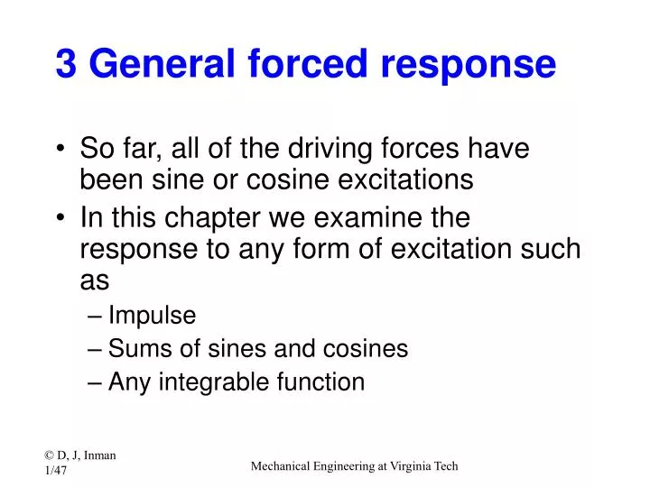
3 General forced response. So far, all of the driving forces have been sine or cosine excitations In this chapter we examine the response to any form of excitation such as Impulse Sums of sines and cosines Any integrable function.

E N D
3 General forced response • So far, all of the driving forces have been sine or cosine excitations • In this chapter we examine the response to any form of excitation such as • Impulse • Sums of sines and cosines • Any integrable function Mechanical Engineering at Virginia Tech
Linear Superposition allows us to break up complicated forces into sums of simpler forces, compute the response and add to get the total solution Mechanical Engineering at Virginia Tech
3.1 Impulse Response Function F(t) Impulse excitation t -e t +e t e is a small positive number Figure 3.1 Mechanical Engineering at Virginia Tech
From sophomore dynamics The impulse imparted to an object is equal to the change in the objects momentum i.e. area under pulse F(t) t -e t +e t Mechanical Engineering at Virginia Tech
We use the properties of impulse to define the impulse function: Dirac Delta function Equal impulses F(t) t Mechanical Engineering at Virginia Tech
The effect of an impulse on a spring-mass-damper is related to its change in momentum. Just before impulse Just after impulse Thus the response to impulse with zero IC is equal to the free response with IC: x0=0 and v0 =FDt/m Mechanical Engineering at Virginia Tech
Recall that the free response to just non zero initial conditions is: Mechanical Engineering at Virginia Tech
x(t) k c m So for an underdamped system the impulse response is (x0 = 0) 1 0.5 h(t) 0 -0.5 -1 0 10 20 30 40 Time Response to an impulse at t = 0, and zero initial conditions Mechanical Engineering at Virginia Tech
The response to an impulse is thus defined in terms of the impulse response function, h(t). Mechanical Engineering at Virginia Tech
1 t=0 0 h1 For example: If two pulses occur at two different times then their impulse responses will superimpose -1 0 10 20 30 40 1 t=10 0 h2 -1 0 10 20 30 40 1 0 h1+h2 -1 0 10 20 30 40 Time Mechanical Engineering at Virginia Tech
Consider the undamped impulse response Mechanical Engineering at Virginia Tech
Example 3.1.1Design a camera mount with a vibration constraint Consider example 2.1.3 of the security camera again only this time with an impulsive load Mechanical Engineering at Virginia Tech
Using the stiffness and mass parameters of Example 2.1.3, does the system stay with in vibration limits if hit by a 1 kg bird traveling at 72 kmh? The natural frequency of the camera system is From equations (3.7) and (3.8) with = 0, the impulsive response is: The magnitude of the response due to the impulse is thus Mechanical Engineering at Virginia Tech
Next compute the momentum of the bird to complete the magnitude calculation: Next use this value in the expression for the maximum value: This max value exceeds the camera tolerance Mechanical Engineering at Virginia Tech
Example 3.1.2: two impacts, zero initial conditions. (double hit) Mechanical Engineering at Virginia Tech
Example 3.1.2 two impacts and initial conditions Note, no need to redo constants of integration for impulse excitation (others, yes) Mechanical Engineering at Virginia Tech
Computation of the response to first impulse: Mechanical Engineering at Virginia Tech
Total Response for 0< t < 4 Mechanical Engineering at Virginia Tech
Next compute the response to the second impulse: Here the Heaviside step function is used to “turn on” the response to the impulse at t = 4 seconds. Mechanical Engineering at Virginia Tech
To get the total response add the partial solutions: Mechanical Engineering at Virginia Tech
xi t ti 3.2 Response to an Arbitrary Input The response to general force, F(t), can be viewed as a series of impulses of magnitude F(ti)Dt Response at time tdue to the ith impulse zero IC xi(t) = [F(ti)Dt ].h(t-ti) for t>ti F(t) Impulses F(ti) (3.12) t ti t1,t2 ,t3 Mechanical Engineering at Virginia Tech
Properties of convolution integrals: It is symmetric meaning: Mechanical Engineering at Virginia Tech
The convolution integral, or Duhamel integral, for underdamped systems is: • The response to any integrable force can be computed with • either of these forms • Which form to use depends on which is easiest to compute Mechanical Engineering at Virginia Tech
Example 3.2.1: Step function input Figure 3.6 Step function To solve apply (3.13): Mechanical Engineering at Virginia Tech
Integrating (use a table, code or calculator) yields the solution: Fig 3.7 Mechanical Engineering at Virginia Tech
m Example: undamped oscillator underIC and constant force For an undamped system: F0 t1 t2 The homogeneous solution is x(t) Good until the applied force acts at t1, then: k 0 Mechanical Engineering at Virginia Tech
Next compute the solution between t1 and t2 Mechanical Engineering at Virginia Tech
Now compute the solution for time greater than t2 0 0 Mechanical Engineering at Virginia Tech
Total solution is superposition: 0.3 0.2 Displacement x(t) 0.1 0 -0.1 0 2 4 6 8 10 Time (s) Mechanical Engineering at Virginia Tech
Example 3.2.3: Static versus dynamic load This has max value of , twice the static load Mechanical Engineering at Virginia Tech
Numerical simulation and plotting • At the end of this chapter, numerical simulation is used to solve the problems of this section. • Numerical simulation is often easier then computing these integrals • It is wise to check the two approaches against each other by plotting the analytical solution and numerical solution on the same graph Mechanical Engineering at Virginia Tech
3.3 Response to an Arbitrary Periodic Input We have solutions to sine and cosine inputs. What about periodic but non-harmonic inputs? We know that periodic functions can be represented by a series of sines and cosines (Fourier) Response is superposition of as many RHS terms as you think are necessary to represent the forcing function accurately 2 T 1.5 1 0.5 0 Displacement x(t) -0.5 -1 -1.5 -2 0 2 4 6 Time (s) Figure 3.11 Mechanical Engineering at Virginia Tech
Recall the Fourier Series Definition: Mechanical Engineering at Virginia Tech
The terms of the Fourier series satisfy orthogonality conditions: Mechanical Engineering at Virginia Tech
Fourier Series Example F(t) Step 1: find the F.S. and determine how many terms you need F0 0 t1 t2=T Mechanical Engineering at Virginia Tech
Fourier Series Example 1.2 1 F(t) 2 coefficients 0.8 10 coefficients 100 coefficients 0.6 Force F(t) 0.4 0.2 0 -0.2 0 0.5 1 1.5 2 2.5 3 3.5 4 4.5 5 Time (s) Mechanical Engineering at Virginia Tech
Having obtained the FS of input • The next step is to find responses to each term of the FS • And then, just add them up! • Danger!!: Resonance occurs whenever a multiple of excitation frequency equals the natural frequency. • You may excite at 100rad/s and observe resonance while natural frequency is 500rad/s!! Mechanical Engineering at Virginia Tech
Solution as a series of sines and cosines to The solution can be written as a summation Solutions calculated from equations of motion (see section Example 3.3.2) Mechanical Engineering at Virginia Tech
3.4 Transform Methods An alternative to solving the previous problems, similar to section 2.3 Mechanical Engineering at Virginia Tech
f(t) F(s) Step function, u(t) e-at sin(w t ) 1/s 1/(s+a) w / ( s2 + w 2) Laplace Transform • Laplace transformation • Laplace transforms are very useful because they change differential equations into simple algebraic equations • Examples of Laplace transforms (see page 216) in book) Mechanical Engineering at Virginia Tech
u(t) t Laplace Transform • Example: Laplace transform of a step function u(t) • Example: Laplace transform of e-at e-at t Mechanical Engineering at Virginia Tech
Laplace Transforms of Derivatives • Laplace transform of the derivative of a function Integration by parts gives, Mechanical Engineering at Virginia Tech
Laplace Transform Procedures • Laplace transform of the integral of a function • Steps in using the Laplace transformation to solve DE’s • Find differential equations • Find Laplace transform of equations • Rearrange equations in terms of variable of interest • Convert back into time domain to find resulting response (inverse transform using tables) Mechanical Engineering at Virginia Tech
Laplace Transform Shift Property Note these shift properties in t and s spaces... thus Mechanical Engineering at Virginia Tech
Example 3.4.3: compute the forced response of a spring mass system to a step input using LT Compare this to the solution given in (3.18) Mechanical Engineering at Virginia Tech
From Fourier series of non-periodic functions Allow period to go to infinity Similar to Laplace Transform Useful for random inputs Corresponding inverse transform Fourier transform of the unit impulse response is the frequency response function Fourier Transform w =2 and M=1 n 0.1 0.05 0 h(t) -0.05 -0.1 0 1 2 3 4 Time (s) 20 10 0 Normalized H(w) (dB) -10 -20 0 1 2 3 4 5 Frequency (Hz) Fourier Transform Mechanical Engineering at Virginia Tech