Query Optimization in Datalog: Formulating and Computing Efficient Queries
550 likes | 654 Views
Learn about query equivalence, view usability, formalism, and program computation in Datalog, a logic-based query language. Understand predicates, rules, assignments, and more.

Query Optimization in Datalog: Formulating and Computing Efficient Queries
E N D
Presentation Transcript
Motivation (1) We have a relation Bus(from, to). Consider the following 2 queries: SELECT DISTINCT B1.from, B2.to FROM Bus B1, Bus B2 WHERE B1.to = B2.from; What do these queries compute? SELECT DISTINCT B1.from, B2.to FROM Bus B1, Bus B2, Bus B3 WHERE B1.to = B2.from and B1.to = B3.from;
Query Equivalence • From looking carefully we can conclude that the queries always return the same values. • Wouldn’t it be nice if any time someone wrote the second query in a database, the first one would be computed instead? (With one less join!!) • Problem: Given a query Q, how can we find the most efficient query Q’ that is equivalent to Q?
Motivation (2) Suppose that we computed the first 2 queries. Can we used its results in order to compute the third query? SELECT S.sid, R.bid FROM Sailors S, Reserves R WHERE S.sid = R.sid; SELECT * FROM Boats B WHERE color = ‘red’; SELECT DISTINCT S.sid FROM Sailors S, Reserves R, Boats B WHERE S.sid = R.sid and R.bid = B.bid and B.color = ‘red’;
View Usability • We can use the first 2 queries to return the third. • Computing the third query using the results of the previous 2 is more efficient then computing it from scratch. • Problem: Given computed queries V1, ..., Vk and a new query Q, can we compute Q using only the results of V1, ..., Vk?
Query Language Formalism • We need a formalism for a query language that allows use to make such analyses. == Datalog (Similar to First Order Logic)
Datalog Program • A Datalog program is a set of rules of the form: p(X1,...,Xn) :- a1(Y1,...,Ym), ..., ak(Z1,...,Zj) • Example: ShortTrip(X, Z) :- Bus(X, Y), Bus(Y, Z) ShortTrip(X, Y) :- Bus(X, Y) Head of the Rule Body of the Rule
Some Definitions • An atom has the form p(Y1,...,Ym) • In the atom above, p is a predicate symbol • A ground atom is an atom that has only constants as arguments. For example: • Bus(‘Jerusalem’, ‘Tel Aviv’) is a ground atom • Bus(‘Jerusalem’, X) is not a ground atom • Bus(Y, X) is not a ground atom • A Datalog rule has a set of atoms in its body and a single atom in its head
More Definitions • A relation is a set of ground atoms for the same predicate symbol. For example: • {Bus(‘Jerusalem’, ‘Tel Aviv’), Bus(‘Tel Aviv’, ‘Haifa’), Bus(‘Ashdod’, ‘Haifa’)} is a relation for the predicate symbol Bus • A database is a set of ground atoms. For example: • {Bus(‘Jerusalem’, ‘Tel Aviv’), Bus(‘Tel Aviv’, ‘Haifa’), Bus(‘Ashdod’, ‘Haifa’), Flight(‘Ben Gurion’, ‘Paris’) }
EDB and IDB Predicates • Given a Datalog program there are 2 types of predicates: • EDB: These are predicates that only appear in the body of rules • IDB: These are predicates that appear in the head of at least one rule • Intuition • EDB: Represent relations in the database • IDB: Represent relations computed from the database
EDB and IDB Example ShortTrip(X, Z) :- Bus(X, Y), Bus(Y, Z) ShortTrip(X, Y) :- Bus(X, Y) LongTrip(X,Z) :- ShortTrip(X,Y), Bus(Y, Z) LongTrip(X,Z) :- ShortTrip(X,Y), ShortTrip(Y,Z) Question: Which predicates are EDB? Which are IDB?
More Definitions • An assignment is a mapping of variables to variables and constants. Assignments can be applied to atoms. • Example: Bus(X,Y) • if f(X) = ‘Jerusalem’, f(Y) = ‘Haifa’, then f(Bus(X,Y)) is Bus(‘Jerusalem’, ‘Haifa’) • if g(X) = Z, g(Y) = Z, then g(Bus(X,Y)) is Bus(Z, Z) • if h(X) = Z, h(Y) = ‘Haifa’, then h(Bus(X,Y)) is Bus(Z, ‘Haifa’)
Applying Assignments • An assignment can also be applied to a rule. An assignment is applied to a rule by applying it to each atom in the rule • Example: r: ShortTrip(X, Y) :- Bus(X, Y) • if f(X) = ‘Lod’, f(Y) = ‘Haifa’, then f(r) is ShortTrip(‘Lod’, ‘Haifa’) := Bus(‘Lod’, ‘Haifa’) • Notation: We sometimes write a rule as H:-B. The application of f to this rule is f(H):-f(B)
Computing a Datalog Program • A set of Datalog rules is called a program. • We can compute a program, given a database that contains ground atoms only for the EDB predicates in the program.
Computing a Datalog Program Compute(P,D) • Result := D • While there are changes to Result do • If there is a rule H:-B in P, and an assignment f to the variables in H and B, such that the all the atoms in f(B) are in Result, then Result := Result f(H)
Example Program: ShortTrip(X, Z) :- Bus(X, Y), Bus(Y, Z) LongTrip(X,Z) :- ShortTrip(X,Y), Bus(Y,Z) Database: {Bus(‘Lod’, ‘Haifa’), Bus(‘Haifa’, ‘Tel Aviv’), Bus(‘Tel Aviv’, ‘Eilat’)}
Before While Loop Program: ShortTrip(X, Z) :- Bus(X, Y), Bus(Y, Z) LongTrip(X,Z) :- ShortTrip(X,Y), Bus(Y,Z) Database: {Bus(‘Lod’, ‘Haifa’), Bus(‘Haifa’, ‘Tel Aviv’), Bus(‘Tel Aviv’, ‘Eilat’)} Result: {Bus(‘Lod’, ‘Haifa’), Bus(‘Haifa’, ‘Tel Aviv’), Bus(‘Tel Aviv’, ‘Eilat’)}
Iteration 1 of While Loop Program: ShortTrip(X, Z) :- Bus(X, Y), Bus(Y, Z) LongTrip(X,Z) :- ShortTrip(X,Y), Bus(Y,Z) Database: {Bus(‘Lod’, ‘Haifa’), Bus(‘Haifa’, ‘Tel Aviv’), Bus(‘Tel Aviv’, ‘Eilat’)} Result: {Bus(‘Lod’, ‘Haifa’), Bus(‘Haifa’, ‘Tel Aviv’), Bus(‘Tel Aviv’, ‘Eilat’), ShortTrip(‘Lod’, ‘Tel Aviv’)} Rule 1: X=‘Lod’ Y=‘Haifa’ Z=‘Tel Aviv’
Iteration 2 of While Loop Program: ShortTrip(X, Z) :- Bus(X, Y), Bus(Y, Z) LongTrip(X,Z) :- ShortTrip(X,Y), Bus(Y,Z) Database: {Bus(‘Lod’, ‘Haifa’), Bus(‘Haifa’, ‘Tel Aviv’), Bus(‘Tel Aviv’, ‘Eilat’)} Result: {Bus(‘Lod’, ‘Haifa’), Bus(‘Haifa’, ‘Tel Aviv’), Bus(‘Tel Aviv’, ‘Eilat’), ShortTrip(‘Lod’, ‘Tel Aviv’), LongTrip(‘Lod’, ‘Eilat’)} Rule 2: X=‘Lod’ Y=‘Tel Aviv’ Z=‘Eilat’
Iteration 3 of While Loop Program: ShortTrip(X, Z) :- Bus(X, Y), Bus(Y, Z) LongTrip(X,Z) :- ShortTrip(X,Y), Bus(Y,Z) Database: {Bus(‘Lod’, ‘Haifa’), Bus(‘Haifa’, ‘Tel Aviv’), Bus(‘Tel Aviv’, ‘Eilat’)} Result: {Bus(‘Lod’, ‘Haifa’), Bus(‘Haifa’, ‘Tel Aviv’), Bus(‘Tel Aviv’, ‘Eilat’), ShortTrip(‘Lod’, ‘Tel Aviv’), LongTrip(‘Lod’, ‘Eilat’), ShortTrip(‘Haifa’, ‘Eilat’)} Rule 1: X=‘Haifa’ Y=‘Tel Aviv’ Z=‘Eilat’
Finished! Program: ShortTrip(X, Z) :- Bus(X, Y), Bus(Y, Z) LongTrip(X,Z) :- ShortTrip(X,Y), Bus(Y,Z) Database: {Bus(‘Lod’, ‘Haifa’), Bus(‘Haifa’, ‘Tel Aviv’), Bus(‘Tel Aviv’, ‘Eilat’)} Result: {Bus(‘Lod’, ‘Haifa’), Bus(‘Haifa’, ‘Tel Aviv’), Bus(‘Tel Aviv’, ‘Eilat’), ShortTrip(‘Lod’, ‘Tel Aviv’), LongTrip(‘Lod’, ‘Eilat’), ShortTrip(‘Haifa’, ‘Eilat’)}
Understanding the Intuition • A rule of the form H:-B means If B is true then H is true • Given the relation Sailors(sname, sid, rating, age), the following query finds the names of all the sailors: name(n):-Sailors(n, i, r, a)
Understanding the Intuition • How can we find the names of the Sailors who have the same rating as their age? • What does the following rule compute? name(sn):-Sailors(sn, si, r, a), Reserves(si, bi, d), Boats(bi, bn, ‘red’)
Unsafe Rules • How can we compute the following rule? CanGo(X, Y):- Bus(X, ‘Jerusalem’) • Suppose our database is the fact {Bus(‘Haifa’, ‘Jerusalem’)} • By definition, our result can contain: {CanGo(‘Haifa’, ‘Jerusalem’), CanGo(‘Haifa’,’Lod’), CanGo(‘Haifa’,’Taiwan’)....}
The Problem • We can assign Y any value. It does not depend on the facts in the database. The values returned depend only on the domain to which we are mapping. • The active domain of a program P, given a database D is the set of constants appearing in P and D. We denote this set by: Active(P,D)
The Solution • Definition: A Datalog program P is domain independent if for all databases D, the result of computing P with respect to a domain containing Active(P,D) is the same as the result of computing P with respect to Active(P,D). • Intuition: If a program is domain independent we only have to try assignments that map variables to constants in the Active domain. Nothing else will yield additional results.
Safety vs. Domain Independence • Safety is a syntactic rule that ensures domain independence. • Definition: A Datalog rule is safe if every variable appearing in its head also appears in an atom in its body We will only consider safe programs Domain Independent Programs Safe Programs
Safe Rules: Examples Note that this is a fact, i.e., a rule without a body • Safe: • CanGo(X, Y):- Bus(X, Y) • CanGo(X, Z):- Bus(X, Y), CanGo(Y,Z) • CanGo(‘Haifa’, ‘Haifa’). • CanBuy(X):- ForSale(X), X < 200 • Unsafe: • CanGo(X, Y):- Bus(X, ‘Jerusalem’) • CanGo(X, X). • CanBuy(X):- X < 200
Safe Rules - Algorithm • For safe rules, the algorithm on Slide 16 is finite, since it is enough to try assignments that map variables to constants in the database. • Otherwise, the algorithm would be infinite. We only consider safe rules
Dependency Graph and Recursion • A dependency graph is a graph that models the way that predicates depend on themselves. • Given a program P, the dependency graph of P has: • a node for each predicate in P • an edge from a predicate p to a predicate q if there is a rule with q in the head and p in the body • A recursive predicate in a program P is a predicate that is in a cycle in P’s dependency graph
Example (1) CanGo(X, Y):- Bus(X, Y) CanGo(X, Z):- Bus(X, Y), CanGo(Y,Z) CanGo • CanGo is recursive • Bus is not recursive • What does this program compute? Bus
Example (2) p(X):- r(X), q(X) q(X):- r(X), p(X) q p • Which predicates are recursive? • What does this program compute? r
Expressiveness:Datalog vs. Relational Algebra • We can express queries in Datalog that are not expressible in Relational Algebra. • Example: Transitive closure. (See CanGo predicate) • This is possible because of recursion. • Now we will consider only non-recursive programs. • In this case can we translate queries between Datalog and relational algebra?
Translating RA to Datalog • We start by translating RA queries with SELECT, PROJECT, TIMES, UNION (without MINUS). • Lemma: Every relational algebra expression produces the same relation as some relational algebra expression whose selections are only of the form XYwhere is an arithmetic comparison operator.
Example • Consider: ¬($1=$2 and ($1<$3 or $2<$3)) (R) • Remember DeMorgan’s laws: • ¬(X and Y) = ¬X or ¬Y • ¬(X or Y) = ¬X and ¬Y • So, the expression above is equivalent to ¬($1=$2) or ¬($1<$3 or $2<$3) (R) = ¬($1=$2) or (¬$1<$3 and ¬$2<$3) (R) = ($1<>$2) or ($1>=$3 and $2>=$3) (R)
Example (continued) • Now, or because union and and becomes composition of select. So: • ($1<>$2) or ($1>=$3 and $2>=$3) (R) = • ($1<>$2) (R)U ($1>=$3 and $2>=$3) (R) = • ($1<>$2) (R)U ($1>=$3) ( ($2>=$3) (R)) We did it! From now on we assume all RA expressions are of this form
Translating RA to Datalog (1) • Theorem: Every query expressible in RA without minus is expressible in a non-recursive Datalog program. • Proof: By induction on j the number of operators in the query. • Base j=0: The query is a relation R. Then R is an EDB expression and is “available” without any rules.
Translating RA to Datalog (2) • Assume for queries with j operators. We show for j+1: • Case 1: The expression is E = E1U E2 . Then, by the inductive hypothesis there are predicates e1 and e2 defined by non-recursive Datalog rules whose relations are the same as E1 and E2. Suppose that they have arity n. Then for E we have the rules: e(X1,...,Xn) :- e1 (X1,...,Xn) e(X1,...,Xn) :- e2(X1,...,Xn)
Translating RA to Datalog (3) • Case 2: E=E1x E2 . Then, there are e1 and e2 as before. Suppose that e1 has arity n and e2 has arity m. Then for E we have the rule: e(X1,...,Xn+m) :- e1 (X1,...,Xn), e2(Xn+1,...,Xn+m) • Case 3: E= $i $j (E1). Then, there is e1 as before. Suppose that the arity of e1 is n. Then, for E we have the rule: e(X1,...,Xn) :- e1 (X1,...,Xn), XiXj
Translating RA to Datalog (4) • Case 4: E= i1,..,ik (E1). Then, there is an e1 as before. Suppose that e1 has arity n. Then for E we have the rule: e(Xi1,...,Xik) :- e1 (X1,...,Xn) • We can prove that with the class of Datalog queries seen so far we can’t express MINUS. • We introduce negation in the queries which will allow us to deal with MINUS.
Translation Example • Query: Boat ids of red and green boats: • In RA: • In Datalog:
Negation • We allow negated atoms in the body of a query. • New safety rule: All variables in the query must also appear in non-negated atoms in the body. • Example: CanBuy(X,Y):- Likes(X,Y), ¬Broke(X) Bachelor(X):- Male(X), ¬Married(X, Y)
Topological Ordering • Before we explain how Datalog rules with negation are computed, we recall how to find a topological ordering of the variables in a graph. • Definition: A topological ordering of the nodes of a graph G is an ordering of the nodes in G such that if there is an edge from n to m, then n is before m in the ordering. • Fact: Every acyclic graph has a topological ordering
Finding a Topological Ordering • Algorithm: Find a node n with no incoming edges. Make n the first node in the ordering. Remove n and its out-coming edges. Continue recursively. • Example: Ordering: r, t, q, p, s s p q t r
Notation • We introduce some notation before presenting the algorithm. Suppose that H:-B is a rule, possibly with negated atoms. • Pos(B): the non-negated atoms in B • Neg(B): the negated atoms in B • Suppose that P is a program. • IDB(P) are the IDB predicated in P • Dep(P) is the dependency graph of P
Computing Datalog Programs with Negation Compute(P,D) • Let Q be an ordering of IDB(P) determined by a topological sort of dep(P). • Result := D • While Q is not empty • r := Q.dequeue(); • While there is a rule H:-B in P with r in its head and there is an assignment f to the variables in H and B, such that f(Pos(B)) is contained in Result and there is no atom in f(Neg(B)) that is in Result, then Result := Result f(H)
Example Program: ShortTrip (X, Y) :- Bus(X,Y) ShortTrip(X, Z) :- Bus(X, Y), Bus(Y, Z) LongTrip(X,Z) :- ShortTrip(X,Y), Bus(Y,Z),¬ShortTrip(X, Z) Database: {Bus(1, 2), Bus(2, 3), Bus(3, 4)} Topological Sort of IDB: ShortTrip, LongTrip
Before Outer While Loop Program: ShortTrip (X, Y) :- Bus(X,Y) ShortTrip(X, Z) :- Bus(X, Y), Bus(Y, Z) LongTrip(X,Z) :- ShortTrip(X,Y), Bus(Y,Z),¬ShortTrip(X, Z) Database: {Bus(1, 2), Bus(2, 3), Bus(3, 4)} Result: {Bus(1, 2), Bus(2, 3), Bus(3, 4)}
Iteration for Predicate ShortTrip Program: ShortTrip (X, Y) :- Bus(X,Y) ShortTrip(X, Z) :- Bus(X, Y), Bus(Y, Z) LongTrip(X,Z) :- ShortTrip(X,Y), Bus(Y,Z),¬ShortTrip(X, Z) Database: {Bus(1, 2), Bus(2, 3), Bus(3, 4)} Result: {Bus(1, 2), Bus(2, 3), Bus(3, 4), ShortTrip(1, 2), ShortTrip(2, 3), ShortTrip(3, 4), ShortTrip(1, 3), ShortTrip(2,4)}