but q & f vary 0 - 180 o & 0 - 360 o

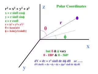
z Polar Coordinates r2 = x2 + y2 + z2 x = r sinqcosf y = r sinqsinf z = r cosq r = (x2 + y2+ z2)½ q = Acos(z/r) f = Asin{y/(rsinq)} r q f x but q & f vary 0 - 180o&0 - 360o dV = dt = r2sinqdrdfdqor ….. dV(shell) = dx • dy • dz = 4pr2sinqdrdfdq y

CM - 2D – Particle on a ring “If a particle is confined to the xy plane, then it has angular momentum along the z axis. angular momentum: Lz = mvr Lz = x • py – y • px E = K + V = K = ½mv2 • (m/m)= p2/2m = Lz2/2mr2 = Lz2/2I moment of inertia: I = mr2

QM - 2D – Particle on a ring “If a particle is confined to the xy plane, then it has angular momentum along the z axis. Ĺz = x • py – y • px= -iħ d( )/df ĤY= Ĺz2/2I Y = -ħ2/2I • d2Y/df2= EY y = Neimf N2 • ∫02p e-imfeimfdf= 1 y = (2p)-1/2eimf E = m2ħ2/2I quantum #, m (or ml ) = 0, ±1, ±2, ±3, ….

2D – Particle on a ring CM E = ½mv2 = p2/2m = J2/2I (I = mr2) QM E = L2/2I (I = mr2) L = hr/l = mlħ l = hr/L E = (mlħ)2/2I moon data m = 7.3 x 1022 kg v = 1,020 m s-1 r = 384000 km 1 revolution = 27.3 days y = (2p)-1/2eimf What is I? What is E (CM)? What is J? What quantum state ml?

Two Particle Problems Goal - Separate problem into 2 distinct one-particle problems. Particle 1: Mass = m1+ m2 Position = center of mass XYZ e.g. X = (m1x1 + m2x2)/(m1 + m2) example: translational motion of diatomic molecule (O2) Particle 2: Mass = m = m1m2/(m1+ m2) Position = position of smaller particle relative to the center of mass use x, y, z or (best) polar coordinates; r, q, f example: rotation of 2 bodies attached at fixed distance (O2)

Two Particle Problems e.g. H2 molecule e.g. H atom m1 = m1 + m2 ~ 2 amu m1 = m1 + m2 ~ 1 amu x = (m1x1 + m2x2)/(m1 + m2) x = (m1x1 + m2x2)/(m1 + m2) x1 = 0 x -1 +1 x1 ~ -1 x -1 +1 m2 = m1m2/(m1 + m2) = ½amu m2 = m1m2/(m1 + m2) ~ me xcm = 0 r2 = ½ bond distance = 0.60 Å xcm ~ -1 = -0.99891 r2 ~ r = 0.529 Å m2 = 1.67 x 1010-24 kg m2 = 9.04 x 10-28 kg

3D – rotations (fixed r) rigid rotor r2 = x2 + y2 + z2 x = r sinqcosf y = r sinqsinf z = r cosq r = (x2 + y2+ z2) q = Acos(z/r) f = Asin{y/(rsinq)} 0 – 180o q 0 - 360o r f dt = r2dr • sinqdq• df ˆ Ĥ= Ĺ2/2I + V Ĺ2 = -ħ2 (d2( )/df2 + cot q d( )/dq + 1/sin2dq d2( )/df2) L = {ℓ(ℓ+ 1)}½ħ Ĺz = -iħ d( )/dfLz= mℓħ Ĥ= -ħ2/2I {d2( )/dq2 + cotq d( )/dq + 1/sin2q d2( )/df2} & cotq = cosq/sinq

Yrot = FmlQl,ml After solving Ĥy= Eroty .... Ĥ= -ħ2/2I {d2( )/dq2 + cotq d( )/dq + 1/sin2q d2( )/df2} Ql,ml associated Legendre polynomials Q0,0= 2-1/2 Q1,0= (3/2)1/2cosq Q1,1= (3/4)1/2 sin q Q2,0= (5/8)1/2 (3cos2q - 1) Q2,1= (15/4)1/2 sin q cosq Q2,2= (15/16)1/2 sin2q Fml= (2p)-1/2 exp(imlf) where l= 0, 1, 2, … ml= -l, - l +1, - l +2, .... + l L = {ℓ(ℓ+ 1)}½ħ Ĺ2 = -ħ2 (d2( )/df2 + cot q d( )/dq + 1/sin2dq d2( )/df2) L = {ℓ(ℓ+ 1)}½ħ Erot = Eq + Ef = {l(l + 1)-ml2}(ħ2/2I) + ml2(ħ2/2I) =l(l + 1)ħ2/2I I = mr2 Ĺz = -iħ d( )/df= mℓħ Lz = mℓħ degeneracy = 2l + 1

Yrot = FmlQl,ml After solving Ĥy= Eroty .... Ĥ= -ħ2/2I {d2( )/dq2 + cotq d( )/dq + 1/sin2q d2( )/df2} Ql,ml associated Legendre polynomials Q0,0= 2-1/2 Q1,0= (3/2)1/2cosq Q1,1= (3/4)1/2 sin q Q2,0= (5/8)1/2 (3cos2q - 1) Q2,1= (15/4)1/2 sin q cosq Q2,2= (15/16)1/2 sin2q Fml= (2p)-1/2 exp(imlf) where l= 0, 1, 2, … ml= -l, - l +1, - l +2, .... + l degeneracy = 2l + 1 Erot = Eq + Ef = {l(l + 1)-ml2}(ħ2/2I) + ml2(ħ2/2I) =l(l + 1)ħ2/2I I = mr2 Eqfor E0,0 = 0 since Q0,0 = 2-1/2 and Erot = 0 + 0 = 0 Eqfor E1,0 = Ĥq = -ħ2/2I [d2( )/dq2+ cot q • d( )/dq]q = Eqq = -ħ2/2I • (3/2)1/2 [d2(cosq)/dq2+ cot q • d(cosq)/dq] = Eqq (cotq = cosq/sinq) = -ħ2/2I • (3/2)1/2 [-1- cosq/sinq• sinq] = (-ħ2/2I • -2) q = ħ2/I • q Eq = ħ2/I and Erot = ħ2/I + 0 = ħ2/I = (+1)ħ2/2I

angular momentum l = 0 mℓ = 0 Ĺ2 = -ħ2 (d2( )/df2 + cot q d( )/dq + 1/sin2dq d2( )/df2) L = {ℓ(ℓ+ 1)}½ħ Ĺz = -iħ d( )/df= mℓħ Yrot = Q • F (spherical harmonics) … is an eigenfunction of the Ĺz and Ĺ2 operators but not Ĺ, Ĺx nor Ĺy. The overall angular momentum scalar value is determined by (Ĺ2)½ . L = 0 Lz = 0 Note that this is not a diagram indicating where the electron may be found. Rather it is a vector diagram representing the limitations on the values of the angular momentum of the electron. The electron with l = 0 (an s orbital) Has no z-component to its angular momentum – it is not confined to a circle.

angular momentum l = 0, 1 Ĺ2 = -ħ2 (d2( )/df2 + cot q d( )/dq + 1/sin2dq d2( )/df2) L = {ℓ(ℓ+ 1)}½ħ Ĺz = -iħ d( )/df= mℓħ L = 21/2 ħ Lz = +1ħ L = 0 Lz = 0 L = 21/2 ħ Lz = -1ħ Yrot = Q • F (spherical harmonics) … is an eigenfunction of the Ĺz and Ĺ2 operators but not Ĺ, Ĺx nor Ĺy. The overall angular momentum scalar value is determined by (Ĺ2)½ .

angular momentum l = 2 L = 61/2 ħ Lz = +2ħ L = 61/2 ħ Lz = +1ħ L = 61/2 ħ Lz = 0 L = 61/2 ħ Lz = -1ħ L = 61/2 ħ Lz = -2ħ

The Hydrogen atom a 3D, 2 particle problem . yNis translational motion of H atom Y = yNye yeis electron motion relative to nucleus Spherical harmonics e(r, q, f)=()()R(r) “Radial function”

e(r, q, f)=R(r)()() • Hamiltonian:Ĥy = Ky + Vy= Ey Force between two charges in vacuum F = q1 • q2/(4peo • r2) (N = kg m s-2) V = F • r = q1 • q2/(4peor)(J = kg m2 s-2) V = -Ze2/(4peor) Applies to H atom and any H-like ion with only 1 e-. K (R(r)()()) Vy • Ĥy = R Q F • -ħ2/2m [1/r2d(r2dy/dr)/dr + 1/(r2sinq) d(sinqdy/dq)/dq+ 1/(r²sin²q) d²y/df²] -Ze2/(4peor) • = Ey

Spherical harmonics ()() These solutions are identical to the rigid rotor model ESH= ħ2l(l+ 1)/2mr2 Ĥ(r, q, f)= Ĥ(ℓ,mℓ()mℓ()) + Ĥ R(r) • Ĥy = -ħ2/2m [1/r2d(r2dy/dr)/dr + 1/(r2sinq) d(sinqdy/dq)/dq + 1/(r²sin²q) d²y/df²] - Ze2/(4peor) • reduces to …… ĤR = -ħ2/2m[1/r2•d(r2dR/dr)/dr + {ħ2l(l+1)/2mr2- Ze2/(4peor)}R

Ĥ R = -ħ2/2m[1/r2•d(r2dR/dr)/dr + {ħ2l(l+1)/2mr2- Ze2/(4peor)}R As the solutions to the Q function already existed in the form of the associated Legendre Polynomials ….. An exact solution to the Hamiltonian for R exists using pre-existing mathematics ….. the associated Laguerre Polynomials • These solutions contain the quantum numbers (n and ℓ) such that …. • n = 1, 2, 3, ….. (principle quantum #) • ℓ = 0, 1, … n – 1 (angular momentum q# as in Q) • mℓ= -ℓ, -ℓ+1, … +ℓ (magnetic quantum number as in F and Q) n,ℓ,mℓ(r, q, f)=ℓ,mℓ()mℓ()Rn,ℓ(r)

R(r) = radial function R = cst *(n-1)th order polynomial in r * e-Zr/2a a = 4peoħ2/me2(units = m) which happens to equal the Bohr orbit radii (0.529Å for H) n,ℓ,mℓ(r, q, f)=ℓ,mℓ()mℓ()Rn,ℓ(r) ĤR = -ħ2/2m [1/r2•d(r2dR/dr)/dr+ {ħ2l(l+1)/2mr2 - Ze2/(4peor)}R = ER E = - Z2e4m/(8eo2h2n2) eq 11.66

What is ynlm? a = 4peoħ2/me2(units = m) y100= 1s = (p-½) • (Z/a)3/2 • exp(-Zr/a) y200= 2s = (32p)-½ • (Z/a)3/2 • {2-(Zr/a)} • exp(-Zr/a) y210= 2pz = (32p)-½ • (Z/a)5/2 • r • exp(-Zr/2a) • (cosq) y211= (64p)-½ • (Z/a)5/2 • r • exp(if) • exp(-Zr/2a) • sinq y21-1= (64p-½) • (Z/a)5/2 • r • exp(-if) • exp(-Zr/2a) • sinq If any 2 wave functions satisfy H and give the same E, then any linear combination of those 2 wave functions (renormalized) will also give the same E. 2px = 2-1/2(y211+ y21-1) 2py= -i2-1/2(y211 - y21-1) 2px = (32p)-½(Z/a)5/2• r • exp(-Zr/2a) • sincos 2py = (32p)-½(Z/a)5/2 • r • exp(-Zr/2a) • sinsin 2pz = (32p)-½(Z/a)5/2 • r • exp(-Zr/2a) • cos

H-atom – Radial Functions 1s 2s 3s

H-atom – Radial Functions 2p 3d 3p

dV = dxdydz dV(cube) = dvxdvydvz = ? dr dV dV = 4p(r+dr)3/3 – 4pr3/3 = 4r2dr 4pr3/3 + 4pr2dr+ 4prdr2 + 4pdr3/3 dV = dxdydz = d = 4pr2dr sin d d

r2R2 1s 3s Probability = r2R2  R2 r2R2 2s r/a Even though the radial function for s orbitals is maximal at r = 0 the r2 term in dt, drops the probability to 0 at the nucleus.

Y1s= (p-½) • (1/a)3/2 • exp(-r/a) rmp= r when d (r2Y1s)dr = 0 = a 1s 3s r2R2 2s r/a

r2R2 3p 2p 3d

Ĥy = -ħ2/2m [1/r2d(r2dy/dr)/dr + 1/(r2sinq) d(sinqdy/dq)/dq + 1/(r²sin²q) d²y/df²] - Ze2/(4peor) = Eyand =E = -Z2e4m/(8eo2h2n2) eq 11.66 eV

e(r, q, f)=()()R(r) Probability = ∫e* e dt =4p ∫r(r+dr) r2R dr• ∫q(q+dq) sin d• ∫f(f+df) d 1 = 4p ∫0∞ r2R dr• ∫0p sin d• ∫02p d = 1 1 1 prob = 4p ∫r(r+dr) r2R dr(over all space)

51 Probability = ∫e* e dt Prob = 4p ∫00.1Å r2R2dr = 4p ∫00.189a r2R2dr R2 = 4/a3 exp(-2r/a) R = 2 (1/a)3/2 exp(-r/a) Prob = 16p/a3∫00.189a r2exp(-2r/a) dr ∫ r2exp(-2r/a) dr= (-ar2 • e-2r/a)/2 – (-a • ò r e-2r/adr) = (-ar2 • e-2r/a)/2 – (-a • a2/4 • e-2r/a • (-2r/a – 1) ]00.189a Prob = 4p • 4/a3[(-ar2 • e-2r/a)/2 – (-a • a2/4 • e-2r/a • (-2r/a – 1)]00.189a

What is an orbital? a one electron spatial wave function The shape of an orbital is the volume enclosed by a surface of constant probability density =  |2| d the size of the orbital depends on confidence level desired. e.g. .... 0r r2R dr * 0psinqQdq * 02p Fdf = 0.9 … says that the probability is 90% of finding e- within the distance r of the nucleus. r is different at different q & f angles for non s orbitals.

y100/1s (p-1/2)(Z/a)3/2 exp(-Zr/a) y200/2s (32p)-1/2(Z/a)3/2 (2-Zr/a) exp(-Zr/2a) y21-1 (64p)-1/2 (Z/a)5/2sinqexp(-if) r exp(-Zr/2a) y211 (64p)-1/2 (Z/a)5/2sinq exp(if) r exp(-Zr/2a) 2px (32p)-1/2(Z/a)5/2 r exp(-Zr/2a) sinqcosf 2py (32p)-1/2(Z/a)5/2 r exp(-Zr/2a) sinqsinf y210/2pz (32p)-1/2(Z/a)5/2 r exp(-Zr/2a) cosq Prob =  |2| d 0r r2R dr * 0psinqQdq * 02p Fdf = 0.9 • (2px)2 (32p)-1(Z/a)5 r2 exp(-Zr/a) sin2qcos2f • (2py)2 (32p)-1(Z/a)5 r2 exp(-Zr/a) sin2qsin2f • (2pz)2 (32p)-1(Z/a)5 r2 exp(-Zr/a) cos2q

Prob:  = 90 &  = 0 r22 r/a 2px 2s 2py & 2pz

Prob:  = 90 &  = 90 r22 r/a 2py 2s 2px& 2pz

Prob:  = 45 &  = 35 2s 2pz 1s r22 2px 2py r/a

angular momentum l = 0 mℓ = 0 Ĺ2 = -ħ2 (d2( )/df2 + cot q d( )/dq + 1/sin2dq d2( )/df2) L = {ℓ(ℓ+ 1)}½ħ Ĺz = -iħ d( )/df= mℓħ Yrot = Q • F (spherical harmonics) … is an eigenfunction of the Ĺz and Ĺ2 operators but not Ĺ, Ĺx nor Ĺy. The overall angular momentum scalar value is determined by (Ĺ2)½ . L = 0 Lz = 0

angular momentum l = 1 mℓ = 0 Ĺ2 = -ħ2 (d2( )/df2 + cot q d( )/dq + 1/sin2dq d2( )/df2) L = {ℓ(ℓ+ 1)}½ħ Ĺz = -iħ d( )/df= mℓħ L = √2ħ Lz = 0 Note that this is not a diagram indicating where the electron may be found. Rather it is a vector diagram representing the limitations on the values of the angular momentum of the electron. The electron with l = 0 (an s orbital) Has no z-component to its angular momentum – it is not confined to a circle.

angular momentum l = 0, 1 Ĺ2 = -ħ2 (d2( )/df2 + cot q d( )/dq + 1/sin2dq d2( )/df2) L = {ℓ(ℓ+ 1)}½ħ Ĺz = -iħ d( )/df= mℓħ L = 21/2 ħ Lz = +1ħ L = 0 Lz = 0 L = 21/2 ħ Lz = -1ħ Yrot = Q • F (spherical harmonics) … is an eigenfunction of the Ĺz and Ĺ2 operators but not Ĺ, Ĺx nor Ĺy. The overall angular momentum scalar value is determined by (Ĺ2)½ .

angular momentum l = 2 L = 61/2 ħ Lz = +2ħ L = 61/2 ħ Lz = +1ħ L = 61/2 ħ Lz = 0 L = 61/2 ħ Lz = -1ħ L = 61/2 ħ Lz = -2ħ

but q & f vary 0 - 180 o & 0 - 360 o