Download
1 / 20
220 likes | 519 Views
Survival Analysis. http://www.isrec.isb-sib.ch/~darlene/EMBnet/. Modeling review. Want to capture important features of the relationship between a (set of) variable(s) and (one or more) responses Many models are of the form g(Y) = f( x ) + error

E N D
Survival Analysis http://www.isrec.isb-sib.ch/~darlene/EMBnet/ EMBnet Course – Introduction to Statistics for Biologists
Modeling review • Want to capture important features of the relationship between a (set of) variable(s)and (one or more) responses • Many models are of the form g(Y) = f(x) + error • Differences in the form of g, f and distributional assumptions about the error term EMBnet Course – Introduction to Statistics for Biologists
Examples of Models • Linear: Y = 0 + 1x + • Linear: Y = 0 + 1x + 2x2 + • (Intrinsically) Nonlinear: Y = x1x2 x3 + • Generalized Linear Model (e.g. Binomial): ln(p/[1-p]) = 0 + 1x1 + 2x2 • Proportional Hazards (in Survival Analysis): h(t) = h0(t)exp(x) EMBnet Course – Introduction to Statistics for Biologists
Survival data • In many medical studies, an outcome of interest is the time to an event • The event may be • adverse (e.g. death, tumor recurrence) • positive (e.g. leave from hospital) • neutral (e.g. use of birth control pills) • Time to event data is usually referred to as survival data – even if the event of interest has nothing to do with ‘staying alive’ • In engineering, often called reliability data EMBnet Course – Introduction to Statistics for Biologists
Censoring • If all lifetimes were fully observed, then we have a continuous variable • We have already looked at some methods for analyzing continuous variables • For survival data, the event may not have occurred for all study subjects during the follow-up period • Thus, for some individuals we will not know the exact lifetime, only that it exceeds some value • Such incomplete observations are said to be censored EMBnet Course – Introduction to Statistics for Biologists
Survival modeling • Response T is a (nonnegative) lifetime • For most random variables we work with the cumulative distribution function (cdf) F(t) (=P(T <= t)) and the density function f(t) (=height of the histogram) • For lifetime (survival) data, it’s more usual to work with the survival function S(t) = 1 – F(t) = P(T > t) and the instantaneous failure rate, or hazard function h(t) = limt->0P(t T< t+t | T t)/ t EMBnet Course – Introduction to Statistics for Biologists
Survival function properties • The survival function S(t) = 1 – F(t) = P(T > t) is the probability that the time to event is later than some specified time • Usually assume that S(0) = 1 – that is, the event is certain to occur after time 0 • The survival function is nonincreasing: S(u) <= S(t) if time u > time t • That is, survival is less probable as time increases • S(t) → 0 as t → ∞ (no ‘eternal life’) EMBnet Course – Introduction to Statistics for Biologists
Relations between functions • Cumulative hazard function H(t) = 0t h(s) ds • h(t) = f(t)/S(t) • H(t) = -log S(t) EMBnet Course – Introduction to Statistics for Biologists
Kaplan-Meier estimator • In order to answer questions about T, we need to estimate the survival function • Common to use the Kaplan-Meier (also called product limit ) estimator • ‘Down staircase’, typically shown graphically • When there is no censoring, the KM curve is equivalent to the empirical distribution • Can test for differences between groups with the log-rank test EMBnet Course – Introduction to Statistics for Biologists
Cox proportional hazards model • Baseline hazard function h0(t) • Modified multiplicatively by covariates • Hazard function for individual case is h(t) = h0(t)exp(1x1 + 2x2 + … + pxp) • If nonproportionality: • 1. Does it matter • 2. Is it real EMBnet Course – Introduction to Statistics for Biologists
Example: Survival analysis with gene expression data • Bittner et al. dataset: • 15 of the 31 melanomas had associated survival times • 3613 ‘strongly detected’ genes EMBnet Course – Introduction to Statistics for Biologists
Average linkage hierarchical clustering unclustered ‘cluster’ EMBnet Course – Introduction to Statistics for Biologists
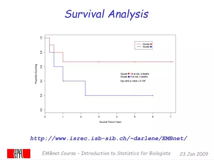
Survival analysis: Bittner et al. • Bittner et al. also looked at differences in survivalbetween the two groups (the ‘cluster’ and the ‘unclustered’ samples) • The ‘cluster’ seemed associated with longer survival EMBnet Course – Introduction to Statistics for Biologists
Kaplan-Meier survival curves EMBnet Course – Introduction to Statistics for Biologists
Average linkage hierarchical clustering, survival samples only unclustered cluster EMBnet Course – Introduction to Statistics for Biologists
Kaplan-Meier survival curves, new grouping EMBnet Course – Introduction to Statistics for Biologists
Identification of genes associated with survival • For each gene j, j = 1, …, 3613, model the instantaneous failure rate, or hazard function, h(t) with the Cox proportional hazards model: h(t) = h0(t)exp(jxij) • and look for genes with both : • large effect size j • large standardized effect size j/SE(j) ^ ^ ^ EMBnet Course – Introduction to Statistics for Biologists
Advantages of modeling • Can address questions of interest directly • Contrast with the indirect approach: clustering, followed by tests of association between cluster group and variables of interest • Great deal of existing machinery • Quantitatively assess strength of evidence EMBnet Course – Introduction to Statistics for Biologists
Survival analysis in R • R package survival • A survival object is made with the function Surv() • What you have to tell Surv • time : observed survival time • event : indicator saying whether the event occurred (event=TRUE) or is censored (event=FALSE) Analyze with Kaplan-Meier curve: survfit, log-rank test: survdiff • Cox proportional hazards model: coxph EMBnet Course – Introduction to Statistics for Biologists