Download
1 / 6
60 likes | 249 Views
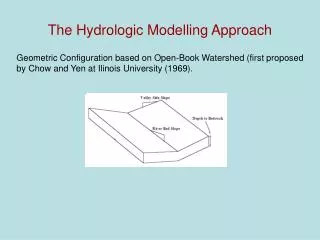
The Hydrologic Modelling Approach. Geometric Configuration based on Open-Book Watershed (first proposed by Chow and Yen at Ilinois University (1969). The Grid-based Process Descriptions.

E N D
The Hydrologic Modelling Approach Geometric Configuration based on Open-Book Watershed (first proposed by Chow and Yen at Ilinois University (1969).
The Grid-based Process Descriptions Excess Rainfall: Calculated using simple mass balance (bucket) approach keeping track of soil moisture storage Overland Flow: Excess rainfall is routed as sheet flow from each grid along the steepest direction – Darcy-Weisbach or Manning’s Equation. River Flow: Lateral inflow from overland is routed using Manning’s Equation (normal depth equation)
Excess Rainfall Calculations s(t) = soil moisture storage p(t) = rainfall; qse(t)= surface flow qss(t)=subsurface flow ET and GW flow can be incorporated if needed
Excess Rainfall Calculations If s(t)> Sf Sf = field capacity qss= 0 if s(t) < Sf L= grid length, β=ground slope, Φ = soil porosity, Ks= Sat. Conductivity if s(t) > Sb Sb= Soil storage capacity=Dφ D= depth to bedrock (depth of soil column) qse= 0 if s(t) < Sb Excess rainfall – Overland Routing – River Routing - Q After Jothityankoon et al., 2002, J. Hydrol.
Excess Rainfall (i) θ L0 Overland Flow and River Flow V Darcy- Weisbach Eqn. Laminar Manning’s Eqn Turbulent After ‘Applied Hydrology’ Chow et al. 1988
Summary of Inputs Static Input: Geophysical Parameters (Distributed): 1. Topography; 2. Soil type (Sf, porosity, Ks), 3. Effective Soil Depth; 4. River bed slope, 5. Channel hydraulic parameters; Minimum calibration – Data available from global databases Dynamic Input: Hydrometeorological Data (Distributed): 1. Rainfall; 2. Initial soil moisture field (and base flow). The Output (what you get for all this): Streamflow at any reach of the river, flow depth, inundation plain.