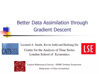
Better Data Assimilation through Gradient Descent
360 likes | 496 Views
This work explores improved data assimilation techniques using Gradient Descent (GD) methodology. We differentiate between perfect model scenarios (PMS) and imperfect model scenarios (IPMS), analyzing how GD outperforms traditional methods like 4DVAR and Ensemble Kalman Filter in both settings. Key results demonstrate how GD facilitates effective assimilation under varied noise conditions while addressing stopping criteria for enhanced performance. Our analysis provides valuable insights into the usefulness of GD for complex dynamical systems, showcasing its potential for better model estimations and error assessments.

Better Data Assimilation through Gradient Descent
E N D
Presentation Transcript
London Mathematical Society - EPSRC Durham Symposium Mathematics of Data Assimilation Better Data Assimilation through Gradient Descent Leonard A. Smith, Kevin Judd and Hailiang Du Centre for the Analysis of Time Series London School of Economics
Outline • Perfect model scenario (PMS) • GD method • GD is NOT 4DVAR • Results compared with Ensemble KF • Imperfect model scenario (IPMS) • GD method with stopping criteria • GD is NOT WC4DVAR • Results compared with Ensemble KF • Conclusion & Further discussion
Ensemble techniques • Generate ensemble directly, e.g. Particle Filter, Ensemble Kalman Filter • Generate ensemble from perturbations of a reference trajectory, e.g. SVD on 4DVAR Gradient Descent (GD) Method K Judd & LA Smith (2001) Indistinguishable States I: The Perfect Model Scenario, Physica D 151: 125-141.
GD is NOT 4DVAR • Difference in cost function • Noise model assumption Observational noise model 4DVAR cost function GD cost function not depend on noise model • Assimilation window 4DVAR dilemma: • difficulties of locating the global minima with long assimilation window • losing information of model dynamics and observations without long window
Reference trajectory Obs t=0 Form ensemble GD result
t=0 Candidate trajectories Form ensemble Sample the local space Perturb observations and run GD
Form ensemble t=0 Ensemble trajectory Draw ensemble members according to likelihood
Obs t=0 Form ensemble Ensemble trajectory
Ensemble members in the state space Compare ensemble members generated by Gradient Descent method and Ensemble Adjustment Kalman Filter method in the state space. Low dimensional example to visualize, higher dimensional results later.
Ikeda Map, Std of observational noise 0.05, 512 ensemble members
Evaluate ensemble via Ignorance Ensemble->p(.) The Ignorance Score is defined by: where Y is the verification. Ikeda Map and Lorenz96 System, the noise model is N(0, 0.4) and N(0, 0.05) respectively. Lower and Upper are the 90 percent bootstrap resampling bounds of Ignorance score
Toy model-system pairs Ikeda system: Imperfect model is obtained by using the truncated polynomial, i.e.
Toy model-system pairs Lorenz96 system: Imperfect model:
Define the implied noise to be and the imperfection error to be Insight of Gradient Descent
Implied noise Imperfection error Distance from the “truth” Statistics of the pseudo-orbit as a function of the number of Gradient Descent iterations for both higher dimension Lorenz96 system-model pair experiment (left) and low dimension Ikeda system-model pair experiment (right).
GD with stopping criteria • GD minimization with “intermediate” runs produces more consistent pseudo-orbits • Certain criteria need to be defined in advance to decide when to stop or how to tune the number of iterations. • The stopping criteria can be built by testing the consistency between implied noise and the noise model • or by minimizing other relevant utility function
Imperfection error vs model error Obs Noise level: 0.01 Model error Imperfection error Not accessible!
Imperfection error vs model error Obs Noise level: 0.002 Obs Noise level: 0.05 Imperfection error
GD vs WC4DVAR WC4DVAR Model error assumption Model error estimates GD
Forming ensemble • Apply the GD method on perturbed observations. • Apply the GD method on perturbed pseudo-orbit. • Apply the GD method on the results of other data assimilation methods. Particle filter?
Imperfect model experiment: Ikeda system-model pair, Std of observational noise 0.05, 1024 EnKF ensemble members, 64 GD ensemble members
Evaluate ensemble via Ignorance The Ignorance Score is defined by: where Y is the verification. Ikeda system-model pair and Lorenz96 system-model pair, the noise model is N(0, 0.5) and N(0, 0.05) respectively. Lower and Upper are the 90 percent bootstrap resampling bounds of Ignorance score
Conclusion • Methodology of applying GD for data assimilation in PMS is demonstrated outperforms the 4DVAR and Ensemble Kalman filter methods • Outside PMS, mmethodology of applying GD for data assimilation with a stopping criteria is introduced and shown to outperform the WC4DVAR and Ensemble Kalman filter methods. • Applying the GD method with a stopping criteria also produces informative estimation of model error. No data assimilation without dynamics.
Thank you! H.L.Du@lse.ac.uk Centre for the Analysis of Time Series: http://www2.lse.ac.uk/CATS/home.aspx




![Better Data, Better Science! [ Better Science through Better Data Management ]](https://cdn3.slideserve.com/6850091/better-data-better-science-better-science-through-better-data-management-dt.jpg)
