A MATLAB Tour of Morphological Filtering
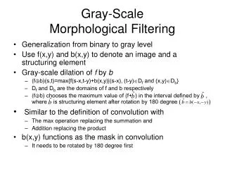
A MATLAB Tour of Morphological Filtering. Dilation. mask B. X. >X=zeros(6,7);X(2:3,4:6)=1;X(4:5,3:5)=1; >se=[0 1;1 1]; >Y=imdilate(X,se);. _. _. Y=X B. Y=X B. Erosion. Erosion. mask B. X. >X=zeros(6,7);X(2:3,4:6)=1;X(4:5,3:5)=1; >se=[0 1;1 1]; >Y=imerode(X,se);.

A MATLAB Tour of Morphological Filtering
E N D
Presentation Transcript
A MATLAB Tour of Morphological Filtering EE465: Introduction to Digital Image Processing
Dilation mask B X >X=zeros(6,7);X(2:3,4:6)=1;X(4:5,3:5)=1; >se=[0 1;1 1]; >Y=imdilate(X,se); EE465: Introduction to Digital Image Processing
_ _ Y=X B Y=X B Erosion Erosion mask B X >X=zeros(6,7);X(2:3,4:6)=1;X(4:5,3:5)=1; >se=[0 1;1 1]; >Y=imerode(X,se); EE465: Introduction to Digital Image Processing
Relationship Between Dilation and Erosion _ ^ =XcB (X B)c >se1=[0 1;1 1]; >se2=fliplr(flipud(se1)); >X1=imdilate((1-X),se2) >X2=1-imerode(X,se1) EE465: Introduction to Digital Image Processing
_ + Opening (X B) B X >X=zeros(6,9);X(3:5,2:4)=1; >X(3:5,6:8)=1;X(5,5)=1;X(2,7)=1 >se=strel('square',3); >Y=imdilate(imerode(X,se),se); %Y=bwmorph(X,’open’); mask B EE465: Introduction to Digital Image Processing
_ + Closing (X B) B X >X=zeros(6,9);X(3:5,2:4)=1; >X(3:5,6:8)=1;X(5,5)=1;X(2,7)=1 >se=strel('square',3); >Y=imerode(imdilate(X,se),se); %Y=bwmorph(X,’close’); mask B EE465: Introduction to Digital Image Processing
Relationship Between Opening and Closing >se=strel('line',10,45); >se2=fliplr(flipud(se)); >X1=~imopen(X,se); >X2=imclose(~X, se2); >isequal(X1,X2) >X1=~imclose(X,se); >X2=imopen(~X, se2); >isequal(X1,X2) EE465: Introduction to Digital Image Processing
_ _ Hit-Miss Operator X B= (X B1)(Xc B2) * >bw = [0 0 0 0 0 0; 0 0 1 1 0 0; 0 1 1 1 1 0; 0 1 1 1 1 0; 0 0 1 1 0 0; 0 0 1 0 0 0] >se = [0 -1 -1; 1 1 -1; 0 1 0]; >bw2 = bwhitmiss(bw,se) X X B * origin mask B1 mask B2 EE465: Introduction to Digital Image Processing
_ Boundary Extraction X=X-(X B) X X • >X=zeros(8,11);X(2:4,4:8)=1;X(5:7,2:10)=1; • > se=strel('square',3); • Y=X-imerode(X,se); %Y=imdilate(X,se)-X; EE465: Introduction to Digital Image Processing
Image Example X X EE465: Introduction to Digital Image Processing
Region Filling Iterations: Pseudo Codes of Region Filling expansion stop at the boundary Y0=P Yk=(Yk-1B)Xc, k=1,2,3… Terminate when Yk=Yk-1,output YkX MATLAB Codes of Region Filling EE465: Introduction to Digital Image Processing
Image Example Y Z >se=strel('square',3); >r=round(size(Y,1)/2); > c=round(size(Y,2)/2); >Z=region_fill(Y,[r,c],se); EE465: Introduction to Digital Image Processing
* Thinning x x x x x x x x x x x x x x x x B5 B6 B7 B8 B4 B1 B2 B3 X0=X Xk=(…( (Xk-1 B1) B2 … B8) where X B=X – X B Stop the iteration when Xk=Xk-1 Question unanswered on the blackboard: For B2,,…,B8, do they operate on Xk-1B1 or Xk-1? EE465: Introduction to Digital Image Processing
MATLAB Implementation function y=thinning(x,iter) se{1}=[-1 -1 -1;0 1 0;1 1 1]; se{2}=[0 -1 -1;1 1 -1;1 1 0]; se{3}=fliplr(rot90(se{1})); se{4}=flipud(se{2}); se{5}=flipud(se{1}); se{6}=fliplr(se{4}); se{7}=fliplr(se{3}); se{8}=fliplr(se{2}); y=x;z=x; for i=1:iter for k=1:8 %y=y&~bwhitmiss(y,se{k}); y=y&~bwhitmiss(z,se{k}); end z=y; end Scheme A Scheme B EE465: Introduction to Digital Image Processing
Which One is Right? Scheme B Original image Scheme A EE465: Introduction to Digital Image Processing
Result by Using BWMORPH Scheme A Scheme B > y=bwmorph(x,’thin’,inf); EE465: Introduction to Digital Image Processing
Summary of Morphological Filtering MATLAB codes circshift(A,z) fliplr(flipud(B)) ~A or 1-A A &~B imdilate(A,B) imerode(A,B) imopen(A,B) imclose(A,B) EE465: Introduction to Digital Image Processing
Summary (Con’d) bwhitmiss(A,B) A&~(imerode(A,B)) region_fill.m bwmorph(A,’thin’); EE465: Introduction to Digital Image Processing
MATLAB Programming Tip #1 • Use functions provided by MATLAB • Although we can implement any function from the scratch, the ones offered by MATLAB are optimized in terms of efficiency and robustness. • If you write your own function, it is safer to use a different name from the prioritized MATLAB function (>which -all) EE465: Introduction to Digital Image Processing
MATLAB Programming Tip #2 • Use as few loops as possible • Example: implementation of histogram calculation • Scheme 1: loop over every position in the image, i.e., i=1-M, j=1-N • Scheme 2: loop over every intensity value, i.e., 0-255 EE465: Introduction to Digital Image Processing