Morphological Simplification
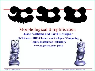
Morphological Simplification. Jason Williams and Jarek Rossignac GVU Center, IRIS Cluster, and College of Computing Georgia Institute of Technology www.cc.gatech.edu/~jarek. Overarching objective. SIMPLIFICATION Understand what it means to simplify a shape or behavior

Morphological Simplification
E N D
Presentation Transcript
Morphological Simplification Jason Williams and Jarek Rossignac GVU Center, IRIS Cluster, and College of Computing Georgia Institute of Technology www.cc.gatech.edu/~jarek
Overarching objective SIMPLIFICATION Understand what it means to simplify a shape or behavior Develop explicit mathematical formalisms independently of any particular domain or representation not stated as the result of some algorithmic process Propose practical implementations MULTI-SCALE ANALYSIS Explore the possibility of analyzing the evolution of a shape or behavior, as it is increasingly simplified, so as to understand its morphological structure and identify/measure its features identify features of interior, boundary, exterior assess their resilience to simplification
Complexity measures for 2D shapes Many measures of complexity are useful in different contexts: • Visibility: Convex, star… number of guards needed • Stabbing: Number of intersections with “random” ray • Wiggles: energy in high frequency Fourier coefficients • Algebraic: Polynomial degree of bounding curves • Fidelity: accuracy required (Hausdorff, area preservation) • Processing: Number of bounding elements • Transmission: compressed file size • Fractal: Fractal dimension • Kolmogorov: Length of data and program We focus primarily on morphological ones: • Sharpness: curvature statistics • Smallest feature size: distance between non adjacent parts of boundary • Topological: Number of components and holes • Non-roundness: perimeter2 /Area
What do we simplify and how much? Simplification replaces a shape by a simpler one • What do we mean by “simpler”? • Informally, we want to • Remove details • Reduce sharpness and wiggles • Eliminate small components and holes • Hence increase the smallest feature size • Shorten (tighten) the perimeter • While minimizing local changes indensity • Ratio of interior points per square unit • How much do we want to simplify • We want to be able to use a geometric measure, r, to specify which of the details should be simplified and how • What does the measure mean? What is the size of a detail?
Restricting simplification to a tolerance zone • We want to restrict all changes to the envelop: tight zone around the boundary bS of the shape S • the yellow fat curve, is the offset (bS)r f bS by r • We further restrict all changes to the Mortar • the green region, is the mortar Mr(bS)=(bSr)r of S • We explain why in the next few slides Mortar Envelop
We need a vocabulary To discuss and to measure simplicity, we need precise terms • We will use three different measures • Smothness (value defined using Differential Geometry) • Regularity (value defined using Morphology) • Mortar (area near the details defined using Morphology) • We want to be able to: • Measure smoothness at every point of the boundary of the shape • Measure regularity at every point in space • Measure the global regularity and smoothness of the whole shape • Define and compute the Mortar for the desired tolerance • Simplify the shape in the Mortar: increasing its regularity & smoothness • A boundary point may be r-smooth or not, r-regular or not
not r-smooth r-smooth r: B A C r-smoothness • A shape S is r-smooth if the curvature of every point B in its boundary bS exceeds r • How to check for r-smoothness at B? • For C2 curves: compare radius of curvature to r • For polygons: estimate radius of curvature • R=v2/(av)z , where v=AC/2 and a=BC–AB • A point may be r-smooth, but not r-regular
Original L is not r-regular Removing the red and adding the green makes it r-regular This shape is r-smooth, but not r-regular r-regularity • A shape S is r-regular if S=Fr(S)=Rr(S) • Fr(S) = Srr, r-Fillet (closing) = area not reachable by r-disks out of S • Rr(S)= Srr, r-Rounding (opening) = area reachable by r-disks in S • Each point of bS can be approached by a disk(r) in S and by oneout of S
Properties of r-regular shapes • Boundary is resilient to thickening by r • bS can be recovered from its rendering as a curve of thickness 2r • One-to-one mapping from boundary to its two offsets by r • The boundary of Sr (resp. Sr) may be obtained by offsetting each point of bS along the outward (resp. inward) normal. No need to trim. • r-regularity implies r-smoothness
When is a point of bS smooth, regular? • How to check for r-regularity at B? • Check whether offset points is at distance r from bS • Dist(B±rN,bS)<r ? • Want a set-theoretic definition? • B is r-regular if it does not lie in the mortar Mr(S) • The mortar is the set of all points that are not r-regular • It is defined in the next slide
Anticore =Fr(S) Mortar (definition) Original set S Fillet: Fr(S) Adds the green Rounding: Rr(S) Removes the red Mortar: Mr(S) = Fr(S) – Rr(S) Core = Rr(S) The plane is divided into core, mortar, and aniticore
Example of Mortar Core Original shape Mortar
Properties of the mortar • All points of the mortar are closer than r to the boundary bS • Restricting the effect of simplification to the mortar will ensure that we do not modify the shape in places far from its boundary • The mortar excludes r-regular regions • Restricting the effect of simplification to the mortar will ensure that regular portions of the boundary are not affected by simplification S Mr(S) M2r(S)
The mortar is the fillet of the boundary • Theorem: Mr(S) is the topological interior of Fr(bS) • Remove lower-dimensional (dangling) portions Mr(S) S i(Fr(bS)) bS
Mr(S) = Fr(S) – Rr(S) Core = Rr(S) Using the Mortar to decompose bS Given r, the regular segments of S are defined as the connected components of r-regular points of bS. • Th1: Regular segment = connected component of bS–Mr(S) • Places where the core and anticore touch • Th2: Irregular segment = connected component of bSMr(S) • Note that irregular points may still be r-smooth Regular segments
Mortar for multi-resolution analysis of space Mr(S) M2r(S) Regularity of a feature indicates its “thickness”
Analyzing the regularity of space • The regularity of a point B with respect to a set S is defined as the minimum r for which B Mr(S) • Points close to sharp features or constrictions are less regular • Different from signed distance field
Morphological Simplifications • Fillet (closing) fills in creases and concave corners • Rounding (opening) removes convex corners and branches • Fillet and rounding operations may be combined to produce more symmetric filters that tend to smoothen both concave and convex features • Fr(Rr(S)) and Rr(Fr(S)) combinations tend to: • Simplify topology: Eliminate small holes and components • Smoothen the shape almost everywhere • Regularize almost everywhere • Increase roundness (by reducingperimeter) • However they • Do not guarantee r-regularity or r-smoothness • Tend to increase or to decrease the density Neither Fr(Rr(S)) nor Rr(Fr(S)) will make this set r-regular
S R2r(S) F2r(S) Fr(S) Rr(S) F2r(R2r(S)) Rr(Fr(S)) R2r(F2r(S)) Fr(Rr(S)) Rounding and filleting combos
Which is better: FR or RF? Removed by rounding S Fr(S) Rr(S) Which option is better? The one that best preserves average density Fr(Rr(S)) Rr(Fr(S))
The Mason filter • We don’t have to make a global choice of FR versus RF • Do it independently for each component of the mortar • The Mason algorithm For each connected segment M of Mr(S) replace MS by MFr(Rr(S)) or by M Rr(Fr(S)), whichever best preservesthe shape i.e., minimizes area of the symmetric difference between original and result “Mason: Morphological Simplification", J Williams, A Powell, and J Rossignac. GVU Tech. Report GIT-GVU-04-05. http://www.gvu.gatech.edu/~jarek/papers.html • Mason preserves density (average area) better than a global Fr(Rr(S))or Rr(Fr(S)), but does not guarantee smoothness nor minimality of perimeter
Mason in Granada S Mortar Mr(S): removed&added Fr(Rr(S)) Mason Rr(Fr(S))
Rr (Fr (S)) Fr (Rr (S)) Mason Mason on a simple shape S
Can we improve on Mason? • Want to ensure r-smoothness • Want to minimize perimeter • Willing to give up some r-regularity • Willing to give up some density preservation • Formulate the solution using a Tight Hull… next slide
Tight Hulls • The tight hull, TH(R,F), of a set R inside a set F is the set H that has the smallest perimeter and satisfies RHF • Extends the idea of a convex hull, CH(R), which may be defined in 2D as the simply connected set that contains R and has smallest perimeter. Hence, CH(R)=TH(R,F) where F is the whole plane. • bH is the shortest path around R in F F R
Related prior art • O(n) algorithm exists based on the Visibility graph • “Euclidean shortest path in the presence of rectilinear barriers”, D.T. Lee and . P. Preparata, Netwirks, 14:393-410, 1984 • “Shortest paths and networks” Joe Mitchell, in Handbook of Discrete and Computational Geometry, Page 610, 2004. • “Shortest Paths in the Plane with Polygonal Obstacles" J Storer and J Reif • Relative convex hull • Jack Sklansky and Dennis F. Kibler. A theory of nonuniformly digitized binary pictures. IEEE Transactions on Systems, Man, and Cybernetics, SMC-6(9):637-647, 1976. • http://www.cs.mcgill.ca/~stever/pattern/MPP/node7.html#SECTION00041000000000000000 • Minimal Perimeter Polygon • Steven M. Robbin, April 97 • http://www.cs.mcgill.ca/~stever/pattern/MPP/talk.html
F R Properties of tight hulls • Let H= TH(R,F) • bH contains the portions of bR that are on the convex hull of R • bRbCH(R) bH • bH is made of some convex portions of bR and of some concave portions of bF joined by short-cuts (straight edges) • Edge (A,B) is a short-cut if A is a silhouette point for B and vice versa.
Computing tight hulls for polygons • Start with CH(R), the convex hull of R • Identify each edge (A,B) of CH(R) that is not on bR and that crosses bF • Compute shortest path from A to B in F–R
Computing tight hulls for smooth shapes • Shortest path • Reasonably easy for shapes bounded by lines and circular arcs. • Track minimum distance field backwards • Propagate constrained distance field from A • Walk back from B along the gradient until you reach A • Constrained curvature flow • Iterative smoothing (contraction) of boundary of Fr(S) while preventing penetration in Rr(S) and in the complement of Fr(S) • Morphological shaving (for discrete representations) • Grow core by adding to it straight line segments of contiguous mortar pixels that start and end at a core pixel
Tightening • The tightening of a shape S is: Tr(S) = TH(Rr(S),Fr(S)) • “Tightening: Perimeter-reducing, curvature-limiting morphological simplification", Jason Williams and Jarek Rossignac. In preparation. S
Topological choices of tightening Invalid ? Invalid ?
Properties of tightenings • bTr(S) is r-smooth • Tr(S) may have irregular parts
The road-tightening problem • By law, the state must own all land located at a distance less or equal to r from a state road. • The states owns an old road C and wants to make it r-smooth so it becomes a highway. • Can it do so without purchasing any new land? • For simplicity, assume first that C is a manifold closed loop.
The road-tightening solution • Let S be the area enclosed by C. • The new road will be bTr(S). • With some restrictions on C, we can extend this result to open road segments.
Comparisons simplified shapes R(F(S)) F(R(S)) mason tightening
FR, RF, mason, tightening red = R(F(S)) cyan = Mortar Blue = Tightening brown = Mason Yellow = Core Green = F(R(S))
Summary and future work • We propose to measure simplicity by regularity and smoothness • Defining regularity for all points of space will support a multi-resolution analysis of shape (interior, boundary, exterior) • We restrict simplifications to the mortar, ensuring that regular areas are preserved • Mason improves on FR and RF combos by better preserving density • Tightening improves on Mason by minimizing perimeter and guaranteeing r-smoothness • We have applied it to the tightening of curves • Future plans • Multi-resolution shape analysis and segmentation using regularity • Higher dimensions: surfaces, volumes, animations