Optimal Linear Fit: Ordinary Least Squares Method
Learn how to determine the best linear fit model for data using the Ordinary Least Squares method, minimizing squared residuals for precise results. Explore the process step by step with detailed explanations and examples. Understand the concept behind selecting the least squares approximating line and polynomial with clear illustrations and calculations. Enhance your understanding of linear regression with this comprehensive guide.


Optimal Linear Fit: Ordinary Least Squares Method
E N D
Presentation Transcript
Background • When we do a study of data and are looking at the relationship between 2 variables, and have reason to believe that a linear fit is appropriate, we need a way to determine a model that gives the optimal linear fit (one that best reflects the trend in the data). • Ex. Relationship between hits and RBI’s • A perfect fit would result if every point in the data exactly satisfied some equation y = a + bx , but this is next to impossible -- too much variability in real world data.
So what do we do? • Assume y = a + bx is the best fit for the data. • Then we can find a point on the line, (xi, f(xi)), with the same x-value as each of the points in the data set, (xi,yi) • Draw a diagram on the board. • Then we say di = yi - f(xi) = distance from point in the data to the point on the line. • di is also called the error or residual at xi -- how far data is from line • So to measure the fit of the line, we could add up all the errors, d1 + d2 + … + dn • However, note that a best fit line will have some data above and some below, so this error will turn out to be 0.
So what do we do? • Therefore, we need to make all of our errors positive by taking either |di| or di2. • |di| will give the same weight to large and small errors, where di2 gives more weight to larger errors • Ex d’s: {0,0,0,0,50} vs {10,10,10,10,10} avg of |di| = 10 = 10
Which one is a better fit? • Which should be considered a better fit? • graph that goes right through 4 points, but nowhere near #5 • graph that is same distance from each point (yes) • |di| method will not show this, but di2 method will.
Ordinary Least Squares Method • So, we will select the model which minimizes the sum of squared residuals: • S = d12 + d22 + … + dn2 = [y1 - f(x1)]2 + …+ [yn - f(xn)]2 • This line is called the least squares approximating line • We can use vectors to help us choose y = a + bx to minimize S
Ordinary Least Squares Method • S, which we will minimize, is just the sum of the squares of the entries in the matrix, Y-MZ. • If n = 3, then Y-MZ is a vector = Then S = || Y-MZ||2
Ordinary Least Squares Method S = || Y-MZ||2 Recall Y and M are given since we have 3 data points to fit. We simply need to select Z to minimize S. Let P be the set of all vectors MZ where Z varies:
Ordinary Least Squares Method It turns out that all of the vectors in set P lie in the same plane through the origin (we discuss why later in the book). The equation of the plane is Take a=0,b=1, or a,b=0 and find that this plane contains: And the normal vector will be U x V =
Ordinary Least Squares Method Y YY-MA O MZMA Recall that we are trying to minimize S = || Y-MZ||2 Y = (y1,y2,y3) is a point in space, and MZ is some vector in the set P which we have illustrated as a plane. S = || Y-MZ||2 is the squared distance from the point to the plane, so if we can find the point,MA, in the plane closest to Y, we will have our solution.
Ordinary Least Squares Method Y YY-MA O MZMA Y-MA is orthogonal to all vectors,MZ, in the plane, so (MZ) • (Y-MA) = 0 Note this rule for dot products when vectors are written as matrices:
Ordinary Least Squares Method Y YY-MA O MZMA 0 = (MZ) • (Y-MA) =(MZ)T(Y-MA)=ZTMT(Y-MA) =ZT(MTY-MTMA) = Z • (MTY-MTMA) The last dot product is in two dimensions and tells that (MTY-MTMA) is orthogonal to every possible Z which can only happen if (MTY-MTMA) = 0,so MTY=MTMA called the normal equations for A
Ordinary Least Squares Method Y YY-MA O MZMA With x1, x2,x3 all distinct, we can show that MTM is invertible, so from MTY=MTMA ,we get A = (MTM)-1MTY, This will give us A=(a,b) which will give then give us the point (a+bx1,a+bx2,a+bx3) closest to Y. Thus the best fit line will then be y=a + bx.
Ordinary Least Squares Method Y YY-MA O MZMA Recall that this argument started by defining n=3 so that we could use a 3 dimensional argument with vectors. The argument becomes more complex, but does extend to any n.
Theorem 1 • Suppose that n data points (x1,y1),…,(xn,yn) of which at least two x’s are distinct. If Then, the least squares approximating line has equation y=a0 + a1x where A = is found by Gaussian elimination from the normal equations MTY=MTMA Since at least two x’s are distinct, MTM is invertible so A=(MTM)-1MTY
Example • Find the least squares approximating line for the following data: (1,0),(2,2),(4,5),(6,9),(8,12) • See what you get with the TI83+
Example • Find an equation of the plane through P(1,3,2) with normal (2,0,-1).
We extend further... We can generalize to select the least squares approximating polynmial of degree m: f(x)=a0+a1x+a2x2+…+anxn where we estimate the a’s
Theorem 2 (proof in ch 6) If n data points are given with at least m+1 x’s distinct, then Then least squares approximating polynomial of degree m is: f(x)=a0+a1x+a2x2+…+anxn where Is found by Gaussian elim from normal equations MTY=MTMA Since at least m+1 x’s are distinct, MTM is invertible so A=(MTM)-1MTY
Note • we need at least one more data point than the degree of the polynomial we are trying to estimate. • I.e. With n data points, we could not estimate a polynomial of degree n.
Example • Find the least squares approximating quadratic for the following data points: (-2,0),(0,-4),(2,-10),(4,-9),(6,-3)
Background Sometimes a system will not have a solution, but we may be able to find a “best approximation” of a solution. Consider A(mxn) and B(mx1) such that AX=B (a system of m equations in n variables). If Z is (nx1), then AZ is (mx1) and ||B-AZ|| is a measure of the distance from B to AZ. So what we might ask is whether there is a column Z that is closest to the solution to AX=B (ie a Z which minimizes ||B-AZ|| over all of the possible columns in n)
More background It turns out that the projection theorem guarantees that such a Z exists: Let U = {AX | Xn} so that U is a subspace of m. We want to find AX in U that is closest to B. The solution is AZ = projU(B) based on projection theorem. Calculation requires: 1) orthogonal basis of U 2) get AZ, need to calculate Z. Recall that (B - AZ) will be in U and so is orthogonal to every vector AX in U.
Continued... So 0=(AX)•(B-AZ)=(AX)T(B-AZ)=XTAT(B-AZ) =X•[AT(B-AZ)] for all X in n So AT(B-AZ) is orthogonal to every vector in n So AT(B-AZ) = 0. So ATB=ATAZ called the normal equations for Z. Most efficient way to find Z is by Gaussian elimination.
Theorem 1-Best Approx Thm A (mxn), B in m, AX = B (m equations, n variables) Any solution Z to the normal equations (ATA)Z=ATB is a best approximation to a solution to AX=B in the sense that ||B-AZ|| is the minimum value of ||B-AX|| with X being any vector in n. (Could be multiple solutions.) If the columns of A are LI, then ATA is invertible, and Z is uniquely given by Z = (ATA)-1ATB.
Example There is no solution to the following system, so find the vector Z=[x0 y0]T that best approximates a solution. 3x - y = 4 x +2y= 0 2x +y = 1 1. Write A and determine if the columns are LI (yes in this case) 2. Find ATA and ATB so we can set up normal equations: (ATA)Z= ATB 3. If cols were LI, then Z=(ATA)-1ATB, else row reduction method 4. See how close AZ will be to B (plug in to see result) (Take a look at example 2 on p. 326 as well)
Least Squares Approximation In 4.4, we did not finish proving thm 2 which gave us the general matrix set-up for ordinary least squares regression. Here, start with ordered pairs of data: (x1,y1),…,(xn,yn) Assume related by polynomial of degree m: y = p(x) = r0 + r1x + r2x2 +…+rmxm Given certain estimated values for ri’s, we will have 2 values to pair with each xi: 1) observed yi, and 2) p(xi) calculated based on the estimated ri’s We would like to select the ri’s which minimize the distance between the yi and the p(xi) since that would make our equation best approximate the data.
Least Squares Continued... Then we want to choose r0,…,rn to minimize: ||Y-p(X)|| = [y1-p(x1)]2 + … + [yn - p(xn)]2 The polynomial, p(x), which does this is called the least squares approximating polynomial.
Least Squares Continued... So p(X) = MR (verify) So our job then is to find R in m+1 such that ||Y - MR||2 is minimized.
Theorem 2 (from 4.4) If n data points are given, then 1. If Z is any solution to the normal equations: Then a least squares approximating polynomial of degree m is: 2. If at least m+1 x’s are distinct, MTM is invertible so Z=(MTM)-1MTY (unique)
Proof of thm 2 Theorem 1 proved part 1 of theorem 2, we just need to show now that having at least m+1 distinct implies that columns of M are LI: Suppose: (The usual setup for showing LI.) If p(x) = r0 + r1x + … +rmxm, the above mtx eq’n can be: p(x1)=p(x2)=…=p(xn)=0. Since p(x) is of degree m with at least m+1 distinct x values that make p(x)=0, p(x) has at least m+1 distinct roots. But a polynomial of degree m can only have m distinct roots unless the polynomial is the zero polynomial. So r0=…=rm=0 Thus the columns of M are LI.
Extension What if instead of having data points for x1,…,xn we used functions of the data points: f(x1),…,f(xn) Then f(x) = r0f0(x) + r1f1(x) + … + rmfm(x) Could we find r0,…,rm to minimize ||Y - f(X)||2 ?
Theorem 3 If n data points are given w/ m+1 fn’s f0(x),…,fm(x), then 1. If Z is any solution to the normal equations: Then is the best approx for these data among all fn’s f(x) of form : Since Holds for all ri’s
Theorem 3 - cont 2. If MTM is invertible (rank M = m+1) then Z is uniquely determined by: Z=(MTM)-1MTY Proof: f(X)=MR w/ Only difference here is that instead of the function being squaring, cubing, etc, it could be any function. Choose R to minimize ||Y-MR||2 and Thm 1 applies again.