Expected accuracy sequence alignment
This text explores the concept of aligning sequences for maximum similarity score using the Needleman-Wunsch algorithm. It also introduces a different approach to compute the most accurate alignment based on posterior probabilities and expected accuracy.

Expected accuracy sequence alignment
E N D
Presentation Transcript
Expected accuracy sequence alignment Usman Roshan
Optimal pairwise alignment • Sum of pairs (SP) optimization: find the alignment of two sequences that maximizes the similarity score given an arbitrary cost matrix. We can find the optimal alignment in O(mn) time and space using the Needleman-Wunsch algorithm. • Recursion: Traceback: where M(i,j) is the score of the optimal alignment of x1..i and y1..j, s(xi,yj) is a substitution scoring matrix, and g is the gap penalty
Affine gap penalties • Affine gap model allows for long insertions in distant proteins by charging a lower penalty for extension gaps. We define g as the gap open penalty (first gap) and e as the gap extension penalty (additional gaps) • Alignment: • ACACCCT ACACCCC • AC-CT-T AC--CTT • Score = 0 Score = 0.9 • Trivial cost matrix: match=+1, mismatch=0, gapopen=-2, gapextension=-0.1
Affine penalty recursion M(i,j) denotes alignments of x1..i and y1..j ending with a match/mismatch. E(i,j) denotes alignments of x1..i and y1..j such that yj is paired with a gap. F(i,j) defined similarly. Recursion takes O(mn) time where m and n are lengths of x and y respectively.
Expected accuracy alignment • The dynamic programming formulation allows us to find the optimal alignment defined by a scoring matrix and gap penalties. This may not necessarily be the most “accurate” or biologically informative. • We now look at a different formulation of alignment that allows us to compute the most accurate one instead of the optimal one.
Posterior probability of xi aligned to yj • Let A be the set of all alignments of sequences x and y, and define P(a|x,y) to be the probability that alignment a (of x and y) is the true alignment a*. • We define the posterior probability of the ith residue of x (xi) aligning to the jth residue of y (yj) in the true alignment (a*) of x and y as Do et. al., Genome Research, 2005
Expected accuracy of alignment • We can define the expected accuracy of an alignment a as • The maximum expected accuracy alignment can be obtained by the same dynamic programming algorithm Do et. al., Genome Research, 2005
Example for expected accuracy • True alignment • AC_CG • ACCCA • Expected accuracy=(1+1+0+1+1)/4=1 • Estimated alignment • ACC_G • ACCCA • Expected accuracy=(1+1+0.1+0+1)/4 ~ 0.75
Estimating posterior probabilities • If correct posterior probabilities can be computed then we can compute the correct alignment. Now it remains to estimate these probabilities from the data • PROBCONS (Do et. al., Genome Research 2006): estimate probabilities from pairwise HMMs using forward and backward recursions (as defined in Durbin et. al. 1998) • Probalign (Roshan and Livesay, Bioinformatics 2006): estimate probabilities using partition function dynamic programming matrices
HMM posterior probabilities • Consider the probability of all alignments of sequences X and Y under a given HMM. • Let M(i,j) be the sum of the probabilities of all alignments of X1...i and Y1…j that end in match or mismatch. • Then M(i,j) is given by • We calculate X(i,j) and Y(i,j) in the same way. • We call these forward probabilities: • f(i,j) = M(i,j)+X(i,j)+Y(i,j)
HMM posterior probabilities • Similarly we can calculate backward probabilties M’(i,j). • Define M’(i,j) as the sum of probabilities of all alignments of Xi..m and Yj..n such that Xi and and Yj are aligned to each other. • The indices i and j start from m and n respectively and decrease • These are also called backward probabilities. • B(i,j)=M’(i,j)+X’(i,j)+Y’(i,j)
HMM posterior probabilities • The posterior probability of xi aligned to yj is given by
Partition function posterior probabilities • Standard alignment score: • Probability of alignment (Miyazawa, Prot. Eng. 1995) • If we knew the alignment partition function then
Partition function posterior probabilities • Alignment partition function (Miyazawa, Prot. Eng. 1995) • Subsequently
Partition function posterior probabilities • More generally the forward partition function matrices are calculated as
Posterior probability calculation • If we defined Z’ as the “backward” partition function matrices then
Posterior probabilities using alignment ensembles • By generating an ensemble A(n,x,y) of n alignments of x and y we can estimate P(xi~yj) by counting the number of times xi is aligned to yj.. Note that this means we are assigning equal weights to all alignments in the ensemble.
Generating ensemble of alignments • We can use stochastic backtracking (Muckstein et. al., Bioinformatics, 2002) to generate a given number of optimal and suboptimal alignments. • At every step in the traceback we assign a probability to each of the three possible positions. • This allows us to “sample” alignments from their partition function probability distribution. • Posteror probabilities turn out to be the same when calculated using forward and backward partition function matrices.
Probalign • For each pair of sequences (x,y) in the input set • a. Compute partition function matrices Z(T) • b. Estimate posterior probability matrix P(xi ~ yj) for (x,y) by • Perform the probabilistic consistency transformation and compute a maximal expected accuracy multiple alignment: align sequence profiles along a guide-tree and follow by iterative refinement (Do et. al.).
Experimental results • http://bioinformatics.oxfordjournals.org/content/26/16/1958