Download
1 / 22
220 likes | 372 Views
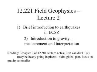
12.221 Field Geophysics – Lecture 2. Brief introduction to earthquakes in ECSZ Introduction to gravity – measurement and interpretation . Reading: Chapter 2 of 12.501 lecture notes (Rob van der Hilst) (may be heavy going in places - skim global part, focus on gravity anomalies. Earthquake.

E N D
12.221 Field Geophysics – Lecture 2 Brief introduction to earthquakes in ECSZ Introduction to gravity – measurement and interpretation Reading: Chapter 2 of 12.501 lecture notes (Rob van der Hilst) (may be heavy going in places - skim global part, focus on gravity anomalies
Earthquake Sequence Joshua Tree M=6.1 April, 1992 Landers M=7.3 June, 1992 Big Bear M=6.2 June, 1992 Hector Mine M=7.1 October, 1999 ? ? ? Magnitude 3 5 6 7 4
Force: f = GmM/r2 G = 6.67 10-11 m3kg-1s-2 Vector directed along r Acceleration of test mass: g = GM/r2 Potential energy: U = -GmM/r Gravitational potential V = GM/r Gravity – simple physics M m r
acceleration potential Gravity – distributed density (x,y,z) Recall Gauss’ theorem: Measuring g places constraints on (x,y,z) Measuring g does not constrain directly (sphere point mass) (x,y,z) can be complicated simple physics, complicated interpretation Interpretation (and effort justified) depend on accuracy of measurements - consider the trade-off judiciously!
Measuring absolute g?Measuring variations in g • f = mg = ku • g ~ 9.8 m/s2 • g ~ 980 cm/ s2 (980 gals - Galileo) • g ~ 1 mgal (10-6) interesting • Need good instrument, good theory!
What causes these variations? Spinning Earth -> centrifugal force, equatorial bulge centrifugal force => less g at equator, no effect at poles equatorial bulge (~elliptical) more mass near equator => g increases r larger at equator => g decreases Dependence of g on latitude () g() = 978032(1 + 0.0052789 sin2 – 0.00000235sin4) mgal Elevation change r -> r + h => g decreases (“free air” effect) Free air correction: g(r+h) = g(r) + (dg/dr) h dg/dr = -2g/r = -0.307 mgal/m
Gravity anomalies In general: g = gobserved – gtheory Free Air theory: gFree Air = g(,h) = g() – 0.307 h Free air anomaly: gfaa = gobserved - gFree Air
Bouguer gravity anomaly:Mountains are not hollow! Approximate as a sheet mass: gBouguer=gFree Air + 2Gh; for = 2.67, 2G = 0.112 mgal/m
Terrain has an effect h in feet!
Tides? www.astro.oma.be/SEISMO/TSOFT/tsoft.html
Step in basement topography g=2G()t[/2+tan-1(x/d)] How big a step makes 0.1 mgal? x d s t b
Example “real-world” problems: • Are the mountains isostatically compensated? • How deep is basin fill in Mesquite basin? • How steep is the basin boundary? • Is Table Mountain a plug or a flow? • Is Black Butte autochthonous? • . . . . . . . . . . . ?
Vidal DEM DEM of Vidal Quadrangle http://data.geocomm.com/dem Rendered using http://www.treeswallow.com/macdem//
Computation of terrain & root using DEM – a new solution to a classic problem Apply Gauss’ theorem & dot product: See http://www.geo-online.org/manuscript/singh99063.pdf for Matlab scripts for carrying out calculations
# # # Southern California Gravity Data (point measurements) # # # # Contributed to the Southern California Earthquake Center by # # Dr. Shawn Biehler of University of California at Riverside # # on December 14, 1998. # # # # Notes: # # 0) Stations name used by Shawn Biehler. # # 1) Latitude and longitude were given to 1/100 minute. Here they are given in # # decimal degrees. # # 2) Elevation is given in meters above sea level. Original was in feet. The # # column 'E' denotes the method of determining elevation: # # T => orginal in tenths of feet (method unspeficied) # # M => map contour (accuracy 1 foot) # # B => bench mark (acurracy 1 foot) # # U => useful (accuracy and method unspecified) # # 3) Raw gravity - 978000.00 mgals (original accuracy 0.01 mgals) # # 4) Predicted gravity - 978000.00 mgals, from XXXXX # # 5) inT -> inner terraine correction, 0 - 1km box. # # outT -> outer terrane correction, 1 - 20 km box. # # T -> method of inner terrane correction. # # 6) FAA - Free Air Anomaly (mgals) (original accuracy 0.01 mgals). # # 7) BOUG -Bouger Anomaly (mgals) (original accuracy 0.01 mgals) # # 8) map - quadrangle map location of stations - first 3 letters denote map, # # digits indicate site marked on map. # # # # stat lat long elev E Raw g Pred g inT outT T faa boug map # #..... ........ .......... ....... . ........ ........ ..... ..... . ....... ....... ......# RO2050 34.96100 -119.44650 889.07 T 1494.47 1742.24 0.32 0.97 G 26.59 828.43 BLC_11 RO2048 34.96667 -119.44000 848.84 T 1498.36 1742.72 0.64 1.08 G 17.59 824.35 BLC_12 RO2020 34.95800 -119.43800 922.29 T 1485.64 1741.98 0.32 1.07 G 28.27 826.49 BLC_10 Gravity data: www.scec.org; on web page