Analyzing Forced Vibration Response Using MATLAB and Bond Graphs in CAMP-G Simulation
This document outlines the analysis of a single degree of freedom system under a force applied to block 2 over a 5-second time frame. It discusses various methods to simulate and visualize the forced vibration response using MATLAB, including manual coding of first-order differential equations, employing SIMULINK, and utilizing CAMP-G for Bond Graph modeling. The most efficient solution is presented as using CAMP-G to automate MATLAB code generation. Key outputs include displacement and momentum plots, showcasing the system's dynamic behavior over time.

Analyzing Forced Vibration Response Using MATLAB and Bond Graphs in CAMP-G Simulation
E N D
Presentation Transcript
ODF Simulation By: Matt Lausmann ME 114 Prof. Granda
The Problem C1 C2 F m1 m2 R1 R2 The problem is to determine how this single degree of freedom system reacts to the force F given to block 2 during a time frame of 5 seconds.
Possible Solutions There are several ways to develop plots to show the forced vibration response. • Develop two (2) 1st order differential equations of motion for the system, and manually write the MATLAB code to produce plots • Use “SIMULINK” to generate a block model and produce the MATLAB code • Employ the use of CAMP-G to produce the MATLAB code through the use of the very powerful MATLAB interface function.
Camp G – Bond Graph By far the easiest solution is to create a Bond Graph model and let the CAMP-G interface tool create the MATLAB code for the plots. The Bond Graph created in CAMP-G is shown below. C R I 1 I C 1 O 1 SE R
Interface - Matlab Once the Bond Graph was created, CAMP-G automatically produces the code and differential equations necessary to produce plots of the vibration response. Three (3) files are produced: • Campgmod.m : contains model parameters, intial conditions, sources and simulation controls • Campgequ.m : contains the system first order differential equations • Campgsym.m : contains the system matrices in symbolic form
Initial Conditions The code does require the user to input some initial conditions. In this problem, the code requires masses for the two blocks, spring and damping constants, starting and ending times, and the source input (force). These are placed wherever red question marks are present in the MATLAB code.
Behind the Scenes When the differential equations are created by CAMP-G in MATLAB, different variables are used to represent displacement, momentum, force, and velocity than we are used to. They are summarized below: q = Displacement p = Momentum e = Force f = Velocity
“P and Q” Plots Besides setting initial conditions, to generate plots of displacement and momentum of the blocks, % signs must be taken out of the generated code. Without doing so, the code remains in “text” format, and is useless. For this problem, displacements and velocities are plotted on the same figure for both blocks and is shown on the next slide. Below is a screenshot of some of the MATLAB code that generates the figures.
P Q Plots (Figure 1) The top row of plots shows the displacement of blocks “1” and “2” vs. time, respectively. The bottom row of plots shows the momentum of blocks “1” and “2” vs. time.
“E and F” Plots Plots for the efforts and flows need additional user input as well. In the campgequ.m file, the time, effort and flow vectors need to be defined. Also, in the campgmod.m file, % marks need to be removed from “text” code for the efforts and flows plots (figure 2). These steps are shown below.
“E and F” Plots (Figure 2) The top plot in this figure shows how the force on block “2” varies with time (from 0-5 seconds) The bottom plot shows how the velocity of block “2” varies with time (from 0-5 seconds)
Conclusion In conclusion, the easiest way to generate plots for the response to the forced vibration in the given system is to employ the use of Bond Graphs in CAMP-G, and let CAMP-G interface with MATLAB to generate the necessary differential equations.