Graphics & Visualization
Graphics & Visualization. Chapter 5 CULLING AND HIDDEN SURFACE ELIMINATION ALGORITHMS. Introduction. Due to restrictions pertaining to our field of view as well as occlusions among the objects, we can only see a tiny portion of the objects that make up our world

Graphics & Visualization
E N D
Presentation Transcript
Graphics & Visualization Chapter 5 CULLING AND HIDDEN SURFACE ELIMINATION ALGORITHMS Graphics & Visualization: Principles & Algorithms Chapter 5
Introduction • Due to restrictions pertaining to our field of view as well as occlusions among the objects, we can only see a tiny portion of the objects that make up our world • Culling algorithms remove primitives that are not relevant to the rendering of a specific frame because: • They are outside the field of view (frustum culling) • They are occluded by other objects (occlusion culling) • They are occluded by front-facing primitives of the same object (back-face culling) • Frustum culling: • Removes primitives that are outside the field of view • Implemented by 3D clipping algorithms Graphics & Visualization: Principles & Algorithms Chapter 5
Introduction (2) • Back-face culling: • Removes primitives that are hidden by front-facing primitives of the same object • Uses normal vectors • The occlusion problem: • Determination of the visible object in every part of the image • Can be solved by computing the first object intersected by each relevant ray emanating from the viewpoint • For correct rendering we must solve the occlusion problem Graphics & Visualization: Principles & Algorithms Chapter 5
Introduction (3) • Numerous Hidden Surface Elimination (HSE) algorithms have been proposed to solve the occlusion problem • Their purpose is to eliminate hidden surfaces of the objects deal with the occlusion problem • HSE algorithms involve sorting of the primitives: • Sorting in the Z (depth) dimension is essential as visibility depends on depth order • Sorting in the X, Y dimensions can accelerate the task of Z sorting, as primitives which do not overlap in X, Y can not possibly occlude each other • HSE algorithms are classified according to their working space: • Object space • Image space Graphics & Visualization: Principles & Algorithms Chapter 5
Introduction (4) • General form of object space HSE: for each primitive { find visible part //(compare against all other primitives) render visible part } • Complexity is O(P2), where P is the number of primitives • General form of image space HSE: for each pixel { find closest primitive render pixel with color of closest primitive } • Complexity is O(pP), where p is the number of image pixels Graphics & Visualization: Principles & Algorithms Chapter 5
Introduction (5) • Computational cost of HSE algorithms is overwhelming despite hardware implementations and parallel processing • Large numbers of primitives can easily be discarded without HSE algorithms • Back-face culling eliminates approximately half of the primitives (back-faces) by a single test at a cost of O(P) • Frustum culling removes those remaining primitives that fall outside the field of view at a cost of O(Pv), where v is the average number of vertices per primitive • Occlusion culling also costs O(P) in the usual case • CONCLUSION: the performance bottleneck are the HSE algorithms which cost O(P2) or O(pP) depending on their working space Graphics & Visualization: Principles & Algorithms Chapter 5
Back-Face Culling • The visible polygons of an object, are those that lie on the hemisphere facing the viewer • If models are constructed in such a way that the back sides of polygons are never visible, then we can cull such polygons. The requirements for this are: • Object surfaces have no boundary (closed) • They are 2D manifolds • They are opaque • Convexity is not a constraint • Back faces can be detected by computing the angle formed by a polygon’s normal vector (pointing outwards from the opaque solid) and the view vector Graphics & Visualization: Principles & Algorithms Chapter 5
Back-Face Culling (2) • If angle > 90o then then the polygon is a back face • The back-face test uses the inner product of the vectors : • Back face culling is extremely effective as it eliminates about 50% of the polygons • Since the back face test and the computation of the normal and view vectors for each polygon take constant time, the complexity is O(P), where P is the number of polygons Graphics & Visualization: Principles & Algorithms Chapter 5
Frustum Culling • The viewing transformation defines the field of view of the observer • The field is restricted by a minimum and maximum depth value, defining a 3D solid called view volume or view frustum • The form of the frustum varies: • Truncated pyramid {perspective projection} • Rectangular parallelepiped {orthographic or parallel projection} • Objective is to eliminate primitives outside the view volume • Takes place after the transformation from ECS to CSS, before the division by w (for perspective projection) • Frustum culling must be performed in 3D space using 3D clipping Graphics & Visualization: Principles & Algorithms Chapter 5
Frustum Culling (2) • Objects to be clipped: • Points • Line segments • polygons • Point clipping is trivial • Line segment and polygon clipping reduce to the computation of a line segment with the planes of the clipping object • In 3D, the interior of the clipping object is defined as: (1) Graphics & Visualization: Principles & Algorithms Chapter 5
Frustum Culling (3) • In orthographic or parallel projection we use matrix which maps the clipping planes to -1 and 1 so that: • In perspective projection, the matrix (before the division by w) maps the clipping planes to –w and w so that: • The value of w is not constant (equal to a point’s ) • Clipping against w is called homogeneous clipping Graphics & Visualization: Principles & Algorithms Chapter 5
Frustum Culling (4) • For a parametric line segment: l(t) = (1-t)p1 + tp2 from p1 = [x1, y1, z1, w1]T to p2 = [x2, y2, z2, w2]T , the value of w can be interpolated as : (1-t)w1 + tw2 then the inequalities (1) can be used to define the part of the line segment within the clipping object: (2) Graphics & Visualization: Principles & Algorithms Chapter 5
Frustum Culling (5) • Solving the 6 inequalities for t we get the 6 intersection points of the line segment with the clipping object planes: (3) Graphics & Visualization: Principles & Algorithms Chapter 5
3D Clipping Algorithms • Most 2D clipping algorithms extend easily to 3D space by addressing: • The intersection computation • The inside / outside test 3D Cohen – Sutherland Line Clipping • In 3D, 6 bits are used to code the 27 partitions of 3D space defined by the view frustum planes: Graphics & Visualization: Principles & Algorithms Chapter 5
3D Clipping Algorithms (2) • A 6-bit code can be assigned to a 3D point according to which of the 27 partitions of 3D space it lies in • Let c1, c2be the 6-bit codes of the endpoints p1, p2 of a line segment: • If accept line segment • If reject line segment • 3D CS pseudocode: CS_Clip_3D ( vertex p1, p2 ) { int c1, c2; vertex I; plane R; c1 = mkcode (p1); c2 = mkcode (p2); if ((c1 | c2) == 0) /* p1p2 is inside */ else if ((c1 & c2) != 0) /* p1p2 is outside */ else { R = /* frustum plane with (c1 bit != c2 bit) */ i = intersect_plane_line (R, (p1,p2)); if outside (R, p1) CS_Clip_3D(i, p2); else CS_Clip_3D(p1, i);} } Graphics & Visualization: Principles & Algorithms Chapter 5
3D Clipping Algorithms (3) • Differs from the 2D algorithm in the: • intersection computation • outside test • Intersection computation: • A 3D plane-line intersection computation is used instead of a 2D line-line intersection computation • The clipping limits are not given in the pseudocode: • In orthographic or parallel projection, these are constant planes and plane-line intersection algorithms are used • In perspective projection and homogeneous coordinates, the plane-line intersections of equations (3) are used • Outside test: • Can be implemented by a sign test on the evaluation of the plane equation R with the coordinates of p1 Graphics & Visualization: Principles & Algorithms Chapter 5
3D Clipping Algorithms (4) 3D Liang – Barsky Line Clipping • The line segment to be clipped is represented by its starting and ending points p1 and p2 (as before) • In orthogonal or parallel projection, the clipping object is a cube and the LB computations extend directly to 3D by adding a z-coordinate inequality: • For perspective projection and homogeneous coordinates, we use the inequalities (2) which define the part of the a parametric line segment within the clipping object: Graphics & Visualization: Principles & Algorithms Chapter 5
3D Clipping Algorithms (5) • These inequalities have the common form tpi ≤ qi for i= 1,2,…,6 where: • Notice that the ratios (qi / pi) correspond to the parametric intersection values of the line segment with clipping plane i • The rest of the LB algorithm remains as in 2D Graphics & Visualization: Principles & Algorithms Chapter 5
3D Clipping Algorithms (6) 3D Sutherland – Hodgman Polygon Clipping • In 3D the clipping object is a convex volume, the view frustum, instead of a convex polygon • The algorithm consists of 6 pipelined stages, one for each face of the view frustum • Main differences against the 2D algorithm are: • The inside_test subroutine must be altered so that it tests whether a point is on the inside half-space of a plane equivalent to testing the sign of the plane equation for the coordinates of the point • The intersect_lines subroutine must be replaced by intersect_plane_line to compute the intersection of a polygon edge against a plane of the clipping volume equations (3) are used for perspective projection Graphics & Visualization: Principles & Algorithms Chapter 5
Occlusion Culling • Occlusion culling discards primitives hidden by other primitives nearer to the observer • Aims at efficiently discarding a large number of primitives before computationally expensive HSE algorithms are applied • Visible set is the subset of primitives that are rendered on at least one pixel of the final image • Occlusion culling algorithms compute a tight superset of the visible set so that the rest of the primitives can be discarded • This superset is called potentially visible set (PVS) • Occlusion culling does not expend time in determining exactly which parts of the primitives are hidden HSE algorithms do • Instead it determines which primitives are entirely NOT visible and quickly discards those, computing the PVS Graphics & Visualization: Principles & Algorithms Chapter 5
Occlusion Culling (2) a (a) visible set (b) all primitives (c) PVS Graphics & Visualization: Principles & Algorithms Chapter 5
Occlusion Culling (3) • PVS is then passed to HSE algorithms • Occlusion culling costs O(P), where P is # of primitives • Two main categories of occlusion culling: • From-point occlusion culling: • Solve the occlusion problem for a single viewpoint • Suitable for outdoor scenes • From-region occlusion culling: • Solve the occlusion problem for an entire region of space • Suitable for dense indoor scenes • Suitable for static scenes because of the pre-computation required Graphics & Visualization: Principles & Algorithms Chapter 5
From-Region Occlusion Culling • A number of applications consists of a set of convex regions (cells), connected by transparent portals • Simplest form: scene represented by 2D floor plan and cells and portals are parallel to either x or y • Primitives are only visible between cells via portals • Cell ca may be visible from cell cb via cell cm, if appropriate sightlines exist that connect their portals • Algorithm requires a pre-processing step • Its cost is only paid once assuming the cells and portals to be static • At pre-processing, a PVS matrix and a BSP tree are constructed • PVS matrix: • Gives the PVS for every cell that the viewer may be in • Visibility is symmetric PVS matrix is symmetric Graphics & Visualization: Principles & Algorithms Chapter 5
From-Region Occlusion Culling (2) • It is constructed, starting from each cell c and recursively visiting all cells reachable from the cell adjacency graph, while sightlines exist that allow visibility from c • Thus the stab tree of c, which defines the PVS of c, is constructed • BSP tree: • Uses separating planes, which may be cell boundaries, to recursively partition the scene • Leafs represent cells • A balanced BSP tree can be used to quickly locate the cell that a point lies in, in O(log2nc) time, where nc is the # of cells • At runtime, the steps that lead to the rendering of the PVS for a viewpoint v are: • 1. Determine cell c of v using the BSP tree • 2. Determine PVS of cell c using PVS matrix • 3. Render PVS Graphics & Visualization: Principles & Algorithms Chapter 5
From-Region Occlusion Culling (3) • Scene modeled as cells and portals (b) Stab trees of the cells (c) PVS matrix (d) BSP tree • PVS does not change while v remains in the same cell • The first 2 steps are only executed when v crosses a cell boundary • At runtime, only the BSP tree and PVS matrix are used Graphics & Visualization: Principles & Algorithms Chapter 5
From-Region Occlusion Culling (4) • Occlusion culling can be optimized by combining it with frustum and back-face culling • Rendering can be restricted to primitives that are both within the view frustum and the PVS • View frustum must be recursively constricted from cell to cell on the stab tree • Pseudocode: main() { determine cell c of viewpoint using BSP tree; determine PVS of cell c using PVS matrix; f = original view frustum; portal render(c, f, PVS); } Graphics & Visualization: Principles & Algorithms Chapter 5
From-Region Occlusion Culling (5) portal render(cell c, frustum f, list PVS); { for each polygon R in c { if ((R is portal) & (c’ in PVS)) { /* portal R leads to cell c’ */ /* compute new frustum f’ */ f’ = clip frustum(f, R); if (f’ <> empty) portal render(c’, f’, PVS); } else if (R is portal) {} else { /* R is not portal */ /* apply back-face cull */ if (!back face(R)) { /* apply frustum cull */ R’ = clip poly(f, R); if (R’ <> empty) render(R’); } } } } Graphics & Visualization: Principles & Algorithms Chapter 5
From-Region Occlusion Culling (6) • f’ = clip frustum(f, R) command computes the intersection of the current frustum f and the volume formed by the viewpoint and the portal polygon R • If this produces odd convex shapes, we may lose the ability to use hardware support • A solution is to replace f’ by its bounding box Graphics & Visualization: Principles & Algorithms Chapter 5
From-Region Occlusion Culling (7) EXAMPLE: • Cell E, that the viewer v lies in, is first determined • Objects in that cell are culled against original frustum f1 • The first portal leading to PVS cell D constricts the frustum to f2 • Objects within cell D are culled against the new frustum • The second portal leading to cell A reduces to frustum f3 • Objects within cell A are culled against f3 frustum • Recursive process stops here as there are no new portal polygons within f3 frustum Graphics & Visualization: Principles & Algorithms Chapter 5
From-Point Occlusion Culling • From-point occlusion culling renders the scene starting from the current cell • Primitives must be visible through the image space projection of the portals, if these fall within the clipping limits • Recursive calls are made for the cells that the portals lead to • At each step the new portals are intersected with the old portals until nothing remains • An overestimate (window) of the intersection of the portals is computed to reduce complexity Graphics & Visualization: Principles & Algorithms Chapter 5
From-Point Occlusion Culling (2) • In outdoor scenes it can not be assumed that the scene consists of cells and portals • Partitioned regions of such scenes would not be coherent, with regard to their occlusion properties • From-point occlusion culling solves the problem for a single viewpoint does not require as much pre-processing as from-region occlusion culling, since PVS is not computed • Main idea behind from-point techniques is the occluder: • Occluder is a primitive, or combination of primitives, that occludes a large number of other primitives (called occludees) with respect to a certain viewpoint • Region of space defined by the viewpoint and the occluder is the occlusion frustum Graphics & Visualization: Principles & Algorithms Chapter 5
From-Point Occlusion Culling (3) • Primitives that lie entirely within the occlusion frustum can be culled • Partial occludees must be referred to the HSE algorithms • Two main steps are required to perform occlusion culling for a viewpoint v: • Create a small set of good occluders for v • Perform occlusion culling using these occluders Graphics & Visualization: Principles & Algorithms Chapter 5
From-Point Occlusion Culling (4) • Planar occluders ranked according to the area of screen space projections were used by Coorg and Teller • Their ranking function is: where A is the area of a planar occluder, is its unit normal vector and is the vector from the viewpoint to the center of the plane occluder • A usual way of computing a planar occluder is as the proxy for a primitive or object • The proxy is a convex polygon perpendicular to the view direction inscribed within the occlusion frustum of the occluder object or primitive Graphics & Visualization: Principles & Algorithms Chapter 5
From-Point Occlusion Culling (5) • Occlusion culling step can be made more efficient by keeping a hierarchical bounding volume description of the scene • Starting at the top level, a bounding volume that is entirely inside/outside an occlusion frustum is rejected/rendered • A bounding volume that is partially inside and partially outside is split into the next level of bounding volumes Graphics & Visualization: Principles & Algorithms Chapter 5
From-Point Occlusion Culling (6) • Simple occlusion culling suffers from the problem of partial occlusion: • An object may not lie in the occlusion frustum of any individual primitive cannot be culled, although it may lie in the occlusion frustum of a combination of adjacent primitives • For this reason algorithms that merge primitives or their occlusion frusta have been developed: • Papaioanou proposed an extension to the basic planar occluder method, called solid occluders, to address the partial occlusion problem, by dynamically producing a planar occluder for the entire volume of an object Graphics & Visualization: Principles & Algorithms Chapter 5
Hidden Surface Elimination • HSE algorithms must provide a complete solution to the occlusion problem • Primitives or parts of primitives that are visible must be rendered directly • HSE algorithms sort the primitives intersected by the projection rays • For occlusion this reduces to the comparison of 2 points: p1=[x1, y1, z1]T and p2=[x2, y2, z2]T • If they are on the same ray then they form an occluding pair the nearer one will occlude the other • There are 2 cases: • Orthogonal projection: assuming that projection rays are parallel to the z-axis, 2 points form an occluding pair if: (x1 = x2) and (y1 = y2) Graphics & Visualization: Principles & Algorithms Chapter 5
Hidden Surface Elimination (2) • Perspective projection: perspective division must be performed to determine if 2 points form an occluding pair. The condition now is: (x1 / z1 = x2 / z2) and (y1 / z1 = y2 / z2) • In perspective projection, the costly perspective division is performed anyway within the ECS to CSS part of the viewing transformation Graphics & Visualization: Principles & Algorithms Chapter 5
Hidden Surface Elimination (3) • It transforms the perspective view volume into a rectangular parallelepiped make direct comparisons of x and y coordinates for the determination of occluding pairs • For this reason HSE takes place after the viewing transformation into CSS • Z coordinates are maintained for the purpose of HSE during the viewing transformations • Most HSE algorithms take advantage of coherence intersection calculations are replaced by incremental computation: • Surface coherence • Object coherence • Scanline coherence • Edge coherence • Frame coherence Graphics & Visualization: Principles & Algorithms Chapter 5
Z – Buffer Algorithm • Initially dismissed because of its high memory requirements • Today a hardware implementation of the Z-buffer algorithm can be found on every graphics accelerator • Algorithm maintains a 2D memory of depth values (Z-buffer), with the same spatial resolution as the frame buffer • 1:1 correspondence between frame and Z–buffer elements • Every element of the Z-buffer maintains the minimum-depth-so-far for the corresponding pixel of the frame buffer • Z-buffer is initialized to a maximum, usually the far clipping plane • For each primitive, during rendering, we compute (zp, cp) at a pixel p = (xp, yp), where zp is the depth of the primitive at p, and cp its color at p Graphics & Visualization: Principles & Algorithms Chapter 5
Z – Buffer Algorithm (2) frame – buffer Z – buffer 3D scene • Assuming that depth values decrease as we move away from the view point, the main Z-buffer test is: if (z-buffer[xp, yp] < zp) { f-buffer[xp, yp] = cp; /* update frame buffer */ z-buffer[xp, yp] = zp; /* update depth buffer */ } Graphics & Visualization: Principles & Algorithms Chapter 5
Z – Buffer Algorithm (3) • Computation of the depth zp at each pixel that a primitive covers, is an efficiency issue of the Z-buffer algorithm: • Computing the intersection of the ray defined by the viewpoint and the pixel with the primitive is expensive • We take advantage of surface coherence. Let the plane equation of the primitive be: F (x, y, z) = ax + by + cz + d =0 Solving for the depth (z) we get: F’(x, y) = z = - d/c - (a/c)x - (b/c)y F’ is incrementally computed from pixel (x, y) to pixel (x+1, y) since: F’ (x+1, y) – F’ (x, y) = - a/c • By adding the constant first forward difference of F’ in x or y, we compute the depth value from pixel to pixel at a cost of one addition Graphics & Visualization: Principles & Algorithms Chapter 5
Z – Buffer Algorithm (4) • In practice, depth values at vertices of the planar primitive are interpolated across its edges and then across the scanlines • Same argument applies to the color vector • Complexity of Z-buffer algorithm is O(Ps), where P # of primitives and s average # of pixels covered by a primitive • In practice, as P increases, s decreases proportionally O(p), where p # of pixels • Advantages of the algorithm: • Simplicity • Constant performance • Weaknesses of the algorithm: • Difficulty to handle some special effects (transparency) Graphics & Visualization: Principles & Algorithms Chapter 5
Z – Buffer Algorithm (5) • Result has fixed resolution, inherited from its image space nature • Z-fighting: arithmetic depth sorting inaccuracies for wide clipping ranges • Z-buffer computed during a rendering, can be kept and used in various ways: • Allows depth merging of 2 or more images. Suppose (fa, za) and (fb, zb) represent the frame- and Z-buffers of 2 parts of a scene. These can be merged by selecting the part with the nearest depth value at each pixel: for (x=0; x<XRES; x++){ for (y=0; y<YRES; y++) { Fc[x,y] = (Za[x,y]>Zb[x,y])? Fa[x,y]:Fb[x,y]; Zc[x,y] = (Za[x,y]>Zb[x,y])? Za[x,y]:Zb[x,y]; } } Graphics & Visualization: Principles & Algorithms Chapter 5
Z – Buffer Algorithm (6) • Many more computations can be performed using Z-buffer: • Shadow determination • Voxelization • Voronoi computation • Object reconstruction • Symmetry detection • Object retrieval Graphics & Visualization: Principles & Algorithms Chapter 5
BSP Algorithm • Binary Space Partitioning (BSP) is an object space algorithm that uses a binary tree that recursively subdivides space • The node data represent polygons of the scene • Internal nodes split space by the plane of their polygon, so that children on the left subtree are on one side of the plane and children on the right subtree are on the other Graphics & Visualization: Principles & Algorithms Chapter 5
BSP Algorithm (2) • To construct a BSP tree the following algorithm is used: BuildBSP(BSPnode, polygonDB); { Select a polygon (plane) Pi from polygonDB; Assign Pi to BSPnode; /* Partition scene polygons into those that lie on either side of plane Pi, splitting polygons that intersect Pi */ Partition(Pi, polygonDB, polygonDBL, polygonDBR); if (polygonDBL != empty) BuildBSP(BSPnode->Left,polygonDBL); if (polygonDBR != empty) BuildBSP(BSPnode->Right,polygonDBR); } • The selection of the partitioning plane Pi is critical since we would like to create a balanced BSP tree • A plane is therefore selected, that divides the scene in 2 parts of roughly equal cardinality Graphics & Visualization: Principles & Algorithms Chapter 5
BSP Algorithm (3) • During partitioning, polygons that intersect the partitioning plane must be split to enforce the partitioning can be achieved by extending a clipping algorithm to deliver both the “inside” and the “outside” parts of a clipped polygon • BSP trees can be used to display the scene with the hidden surfaces removed • For a viewpoint v and a BSP node, all polygons that lie in the same partition as v cannot possibly be hidden by polygons of the other partition polygons of the other partition should be displayed first Graphics & Visualization: Principles & Algorithms Chapter 5
BSP Algorithm (4) • Pseudocode: DisplayBSP(BSPnode, v); { if IsLeaf(BSPnode) Render(BSPnode->Polygon) else if (v in ‘left’ subspace of BSPnode->Polygon) { DisplayBSP(BSPnode->Right, v); Render(BSPnode->Polygon); DisplayBSP(BSPnode->Left, v); } else/* v in‘right’ subspace of BSPnode->Polygon */ { DisplayBSP(BSPnode->Left, v); Render(BSPnode->Polygon); DisplayBSP(BSPnode->Right, v); } } Graphics & Visualization: Principles & Algorithms Chapter 5
BSP Algorithm (5) • The DisplayBSP algorithm costs O(P) • The BuildBSP algorithm costs O(P2) • The overall complexity of the BSP algorithm is O(P2) • For static scenes, BuildBSP is used once and then, for every new position of the viewpoint, only the DisplayBSP algorithm must run BSP is suitable for static scenes, but NOT suitable for dynamic scenes Graphics & Visualization: Principles & Algorithms Chapter 5
Depth Sort Algorithm • This algorithm sorts polygons according to their distance from the observer and displays them in reverse order (back to front) • Also called painters’ algorithm • Minimum depth value of polygons is used for the sorting: DepthSort(polygonDB); { /* Sort polygonDB according to minimum z */ for each polygon in polygonDB find MINZ and MAXZ; sort polygonDB according to MINZ; resolve overlaps in z; display polygons in order of sorted list; } • Overlaps in z arise when the z extents of polygons overlap the sorting becomes ambiguous as it is not clear which polygon obscures the other cannot perform sorting in some cases Graphics & Visualization: Principles & Algorithms Chapter 5