Download
1 / 1
10 likes | 117 Views
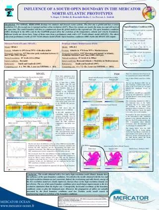
20 %. Annual mean Barotropic Stream Function (BSF). Annual mean Eddy Kinetic Energy (EKE). Annual mean Overturning Stream Function. Annual mean Barotropic Stream Function (BSF). Buffer zone. Radiative OBC. Buffer zone 9N. Buffer zone 9N. Buffer zone 9N. OBC 9N. OBC 9N. OBC 9N.

E N D
20 % Annual mean Barotropic Stream Function (BSF) Annual mean Eddy Kinetic Energy (EKE) Annual mean Overturning Stream Function Annual mean Barotropic Stream Function (BSF) Buffer zone Radiative OBC Buffer zone 9N Buffer zone 9N Buffer zone 9N OBC 9N OBC 9N OBC 9N Buffer zone 20S Buffer zone 20S Buffer zone 20S 9º 70º Non-radiative OBC Buffer Zone 10N 70N 10N 70N 20S 10N 70N Radiative OBC Annual meanSea Surface Height Variance Buffer Zone Radiative OBC INFLUENCE OF A SOUTH OPEN BOUNDARY IN THE MERCATOR NORTH ATLANTIC PROTOTYPES N. Daget, Y. Drillet, R. Bourdallé-Badie, C. Le Provost, L. Siefridt Introduction: For GODAE, MERCATOR develops two analysis and forecast ocean systems. The first one is global and has a coarse resolution (¼º), the second one is regional and has a fine resolution (1/15º). These two systems are nearly the same size and will work at the same time. The south boundary will have to communicate from the global model to the regional one. The open boundary conditions (OBC) developed in the OPA code by the CLIPPER project allow the evolution of the temperature, salinity and velocity boundaries. Different results are shown here. Some of them come from a preliminary study with a 1/3º North Atlantic model (MNATL). The others come from preliminary results of 1/15º North Atlantic model (PAM). Open boundary conditions (OBC) built with MNATL 20S outputs. Open Boundary Condition (OBC) The normal phase velocity used for a variable is : If the normal phase velocity is negative, then the climatologic data are imposed. Mercator North ATLantic (MNATL) Model: OPA8.1 Domain: Atlantic to 20ºS from 70ºN + Gibraltar inflow Horizontal resolution: 1/3º Mercator grid, resolution between 12 and 37 km (358 x 361 pts) Vertical resolution: 43 levels (12 to 200m) Initial conditions : Reynaud Bathymetry: Smith and Sandwell (1997) Computing cost: 4 x 700 Mb, 1 year (on VPP5000) = 10 h Prototype Atlantic Mediterranean (PAM) Model: OPA-8.1 Domain: Atlantic to 9ºN from 70ºN + Mediterranean Horizontal resolution: 1/15º Mercator grid turned in Atlantic, resolution between 5 and 7 km (1288 x 1022 pts) Vertical resolution: 43 levels (6 to 300m) Initial conditions: Reynaud Atlantic + MedAtlas in Mediterranean Bathymetry:Smith and Sandwell (1997) Computing cost: 4 x 7.2 Gb, 1 year (on VPP5000) = 180 h Else If non-radiative OBC are used, the equations become : With : MNATL PAM These two simulations have been forced by 2 perpetual years (mean 1998-2000). One of them (Buffer zone) has a buffer zone. The last one (Radiative OBC) has an open boundary condition built with a mean of the 3 last years of a 10 years MNATL-20S simulation forced by ERA15. Like MNATL, the BSF are comparable among the two simulations ; however, the Gulf Stream is more intense in the OBC simulation. The overturning simulated by OBC is less important than in the buffer simulation. The 10 Sv isoline reaches the boundary in the buffer zone simulation when it is limited to 15N in the OBC simulation. Again, the signal is less noisy close to the boundary. Nevertheless, the more interesting part is the non-radiative OBC simulation presents a very different behaviour. In this case, the 10 Sv isoline reaches only 33N. Consequently, these different simulations show the importance and the advantage of a radiative OBC. The figures below show the SSH variance. The loss of kinetic energy nearby the Cape Hatteras represents an improvement of the model in this area. Moreover, stronger downstream part of the Gulf Stream makes the North Atlantic current well marked. These three simulations have been forced by 10 perpetual years (1998). Two of them have a buffer zone (Buffer zone 9N and Buffer zone 20S). Near the south boundary, there is an important climatologic damping to the temperature and salinity of the Reynaud climatology. The last one (OBC 9N) has an open boundary condition built with a mean of the 3 last years of the MNATL-20S previous simulation. The BSF shows that the solutions are not so different. In the OBC simulation, the overturning stream function increases drastically close to the boundary and the signal is less noisy in the depth. It makes the OBC simulation comparable to the buffer zone at 20S. Similarly, EKE increases in the Caribbean sea. Thanks to the OBC, more information comes into the domain and the Brazil current is better represented. Annual mean Overturning Stream Function The first plot shows the difference of the sea surface EKE between the OBC simulation and the corresponding 9N buffer zone simulation (solid line) and between the OBC simulation and the corresponding 20S buffer zone simulation (dotted line). The EKE increases between 10N and 20N and the OBC simulation gives results comparable to the 20S buffer zone one. The second plot shows the same difference between another kind of OBC simulation and the corresponding buffer zone. This new OBC simulation is forced by ERA15 (mean between 1979 and 1993) and the boundary conditions come from the last 3 years of the corresponding buffer zone simulation. In this case, the differences are very important and the latter OBC simulation is turbulent (at least 20 %). These two latter plots highlight the important role played by the boundary conditions. Cape Hatteras [Buffer Zone] - [Radiative OBC] Conclusion : The results obtained with a low and a high resolution north Atlantic domain show the influence of the open boundary conditions. Nevertheless the results obtained with the low and the high resolution domain are not consistent. Indeed, the overturning and eddy kinetic energy of the low resolution model are clearly improved, whereas those of the high resolution domain are not obvious. The use of the open boundary conditions gives much larger improvements to the low resolution simulation than the higher one. Consequently, horizontal resolution of the boundary conditions seems to play the dominant part. Moreover, the propagation of eddies are actually prevented by the fixed boundary conditions used her. Further works would consist in implementing temporal evolution of the boundary conditions. • Réferences: • Madec G., Delecluse P., Imbard M., Lévy C., 1998: OPA8.1 ocean general circulation model reference manual, Notes du pôle de modélisation IPSL, 11. • Treguier A.M. et al, 2001: An eddy-permitting model of the Atlantic circulation : Evaluation open boudary condition, JGR. • Siefridt L. et al, 2002 : Mise en oeuvre du modèle Mercator à haure résolution sur l’Atlantique nord et la Méditerranée. Mercator Newsletter Nº5