Download
1 / 36
360 likes | 523 Views
Geant4 Milagro Simulation. Vlasios Vasileiou U. Maryland 5/5/2006. Simulation components. The software Corsika – Air shower simulation Geant4 – Simulation of the detector’s response to the EAS particles reaching the ground

E N D
Geant4 Milagro Simulation Vlasios Vasileiou U. Maryland 5/5/2006
Simulation components • The software • Corsika – Air shower simulation • Geant4 – Simulation of the detector’s response to the EAS particles reaching the ground • Milinda – analysis software (among others: adds noise, performs PMT corrections, add time jitter and smears number of pes)
Corsika • Simulates the air showers • Variety of hadronic physics models available • We use • Low energy hadronic model • Fluka 2005 (previously used Gheisha) • High energy hadronic model • Nexus 3 (started using it in the latest Corsika v6.500 with g4sim v2.0). Previously used Venus neXus (NEXt generation of Unied Scattering approach) is a common effort of the authors of VENUS and QGSJET with extensions enabling a safe extrapolation up to higher energies,using the universality hypothesis to treat the high energy interactions . It handlesnucleus-nucleus collisions with an up to date theoretical approach.
Corsika Curved atmosphere (started using it after g4sim v1.2) In the default version of corsika a plane atmosphere is used and the thickness increases as 1/cos(θ). The accuracy of this approximation decreases with θ (for θ=90degthe thickness of the planar atmosphere reaches infinity). Corsika doesn’t allow using θ>70 deg unless a curved atmosphere is selected. How it works: In the curved version the Cartesian coordinate system is kept but the horizontal step size is limited to <20 km.Longer transport distances are divided into appropriate segments to be treated in a local flat atmosphere. After each traversed segment the particle coordinates are transferred into the next local Cartesian coordinate system with its vertical axis pointing to the middle of Earth. Thus the curved Earth's surface is approximated piece by piece by flat segments with limited horizontal extensions.
Geant4 • Geant4 is a simulation toolkit from CERN created for the simulation needs of the LHC. • Biggest advantages • Written in C++ and thus easy to expand & debug. • Wide international collaboration • Far greater functionality and number of physics models than geant3 • New and more accurate physics models • Fewer bugs
g4sim • Milagro simulation code based on Geant4 • Main code written by V. Vasileiou (it’s all my fault...) • C. Lansdell and A. Smith helped with debugging • First beta version out in Summer 2004. • The detector model in the first version of g4sim was almost identical to the one in the g3 version. • Slowly, I rewrote all the code from scratch • Using my own sources for the properties of the detector elements (instead of the numbers in g3). • Rechecking the sizes of the detector elements • Using a different PMT model
g4sim: GeometryThe pond • Source of dimensions a pond schematic from Peter Nemethy. • Support for water over the cover & air under the cover. • Currently using 1cm of water over the cover and no air under the cover. • The layer of air under the cover is uniform all over the water not a good approximation. • In the g3 sim there is no physical cover included in the simulation
g4sim: GeometryThe pond Cover & pond liner • Polypropylene • Diffuse reflector with incidence angle dependent reflectivity. • Calculated from Fresnel’s equations by Geant4 • Have to provide refractive index: 1.49 • Increased reflectivity from the white pipes at the bottom of the pond not included in the simulation. Reflectivity of a flat Water Polypropylene interface for non polarized light.
g4sim: GeometryThe pond cover • Possible problem: Reflectivity from Fresnel’s equations and the results from ’94 David Schmidt’s Milagro memo disagree. UV reflectivity of polypropylene is very low. • More reflections from the cover We trigger more easily by weaker showers. Nhit, npe, mxpe, nfit distributions slightly move to lower values. Reflectivity of a flat Air Polypropylene interface for non polarized light from Fresnel’s equations. Reflectivity of polypropylene (by D. Schmidt) versus the reflectivity of a material assumed to be a perfect reflector. Measurements correspond to some unknown incidence angle.
g4sim: GeometryThe baffles • Baffle dimensions taken from a schematic from M. Schneider • Bug in g4sim v1.2 • Inside part of baffles had the properties of tyvek • True inside part of baffles is made out of the of unknown composition material called “Liner” in D. Schmidt’s memo. • Currently in g4sim v2.0 • Liner is a diffuse reflector with the reflectivity measured by D. Schmidt. • Outside part of baffles: Diffuse reflector with the properties of polypropylene
g4sim: GeometryThe outriggers • Dimensions of outriggers taken from a schematic by Tony Shoup. • They are not all on the same plane (in g3 they are) • They don’t all contain the same amount of water. • In g4 sim their water height takes random values around a mean value. • 76cm ± 10cm • (Thanks to Scott for measuring the water levels of several outriggers.)
g4sim: GeometryThe outriggers • Inside part of outriggers lined with tyvek • Reflections from tyvek a mixture of specular and diffuse • The values of Geant4’s parameters that describe the reflections from Tyvek (sigma_alpha and specular lobe constant) were taken from Auger notes. • Tyvek reflectivity taken from D. Schmidt’s memo
Water properties • Water absorption and scattering lengths • In g3 sim (v3.2 pro?) 18m Absorption length and no scattering • In g4 sim (v0.99 – v1.3), 18m abs length and Rayleigh scattering were mainly used. Simulated other abs lengths too but 18m was always the pro. • g4sim v2.0 • Has both Mie and Rayleigh scattering • Two configurations were mainly used: • Absorption Length 27.4m and Scattering Length 56.8m (Att. Length 19m). Source was an email from Don Coyne to the milagro mailing list dated 5/4/2004. • Absorption length 30m and Scattering length 50m.
Water properties • Rayleigh Scattering – caused be scattering centres smaller than λ/20 • Rayleigh scattering length increases with λ4 and scattering angular distribution goes like ~(1+cosθ2). • Forward and backward scattering probability equal. • Rayleigh scattering very long • Geant4 has code to simulate Rayleigh scattering. Calculates the lengths just for water using the Einstein-Smoluchowski formula
Water propertiesMie scattering • Mie Scattering • Geant4 doesn’t include code for Mie scattering, so I wrote some code to simulate this process • Mie’s angular distribution function is hard to solve • If your scattering centers have similar properties (rindex and size) or if your scattering is dominated by a single species of scatterers • you can approximate the Mie complicated functions that give the scattering angle distribution with a simple function: the Henyey-Greenstein function • Needs only one parameter; the asymmetry factor (g=<cosθ>)
Mie scattering in g4sim v2.0 MC • In the March 2004 Los Alamos meeting Don Coyne presented results of his water scattering measurements. • Showed a plot of relative intensity vs scattering angle • His results would agree with a Henyey-Greenstein function of <cosθ>=0.9999. Extremely forward scattering. • For the g4sim v2.0 MC, I used <cosθ>=0.99
Differential (top) and integral (bottom) plots of the Mie scattering angle distributions for different asymmetry factors.
Water propertiesMie scattering • The asymmetry factor can be calculated if the refractive index and the size of the scatterers is known. • There is a program called MiePlot that performs these calculations (if only we knew what scatters our light in the pond). • Air bubbles, Al2O3, other stuff? • My impression • We will never know what exactly is in our water • For now, just use a conventional very forward asymmetry factor and if any one performs a reliable measurement of the water scattering angular distribution in the future, then try to change things. • For this version of the Mie scattering code • There is no energy dependence of the asymmetry factor • No back-scattering (easy to add, thought about it after I generated all this data)...
PMT properties • Geometry • g4sim v>1.2 uses a full optical model of the PMT • Taken from GLG4SIM generic Geant4 application (G. Horton, D. Motta et al) and modified and bug fixed for Milagro.
PMT model • The PMT model in the G4 Milagro simulation tracks the photons until they are converted tophotoelectrons or until they are absorbed upon incidence on a surface or until they exit the PMT. • Itsimulates reection/refraction/absorption at the glass, photocathode, dynodes and silvered surfaceof the PMT. • The absorption probability of a photon transversing the photocathode material iscalculated using its complex refractive index and thickness. • The probability of a photon detection is a product of the probabilities of the following steps: • The absorption of the photon in the photocathode material and the resulting creation of aphotoelectron • The liberation of the photoelectron in the PMT vacuum • The collection of the photoelectron at the 1st dynode
PMT model • The absorption probability is be calculated from the complex refractive index of the photocathodematerial and depends on the energy and the incidence angle. • Some of the photoelectronsproduced will be liberated into the vacuum and later collected by the 1st dynode. • The probabilityfor a liberated into the vacuum photoelectron to be properly collected by the 1st dynode is calledthe Collection Efficiency of a PMT (CE). • For the PMT model in the simulation the CE is 1; all liberated in the vacuum photoelectrons are detected. And collection efficiency effects are applied later in milinda.
PMT model • Let the liberation probability of a photoelectron into the vacuum be called LP. • The QuantumEfficiency (QE) of a photocathode is defined as the ratio of liberated into the vacuum photoelectronsover the incident on the photocathode photons. • If the probability of a photon being absorbed inthe photocathode is called A then QE = A*LP (1)
PMT model • The LP is only energy dependent, while the A and QE are both energyand incidence angledependent. • The QE data from the spec sheets corresponds to normal incidence, let's call itQEn(E). • The absorption probability at normal incidence, An(E), can be calculated using thecomplex refractive index and the thickness of the photocathode material. • So the LB(E) can becalculated as LB(E) = An(E)/QEn(E) (2) • Deriving LB(E)from (2) and by calculating A(E,θ)we can derive, using (2), the angular dependenceof the quantum efficiency.
PMT tests • I tested some Milagro PMTs • Mainly, made pulse height distributions for different conditions and measured the relative detection efficiency on the surface of the PMT • PMT gain and detection efficiency decrease as we illuminate points far from the top of the photocathode. • I sent a memo out (5/1/2006) about these tests.
PMT tests Pulse height distribution for illumination at different positions of the photocathode . PMT #1024, HV 1800V, PMT vertical
PMT tests Magnetic field effects PMT illuminated at the top
PMT tests Relative detection efficiency Normal illumination at different points of the photocathode. PMT #1024, 1800V, vertical position
PMT tests Relative efficiency vs incidence angle. Illumination of the top of the photocathode under different angles
Milinda’s initial processing of the MC eventNoise addition • The MC event is read by DataRead_MCASCII5 • AddNoise code superimposes noise to the events • Cosmic ray noise • Simulated 5 GeV – 100 TeV , 90deg zenith angle protons thrown uniformly on the pond with cores distributed to +-5km. Kept events with any pmts hit and at most 10AS PMTs hit. Saved in the config_milagro/noise.dat file • Milinda adds, randomly in time, events from this file until the hit rate of the AS tubes becomes 20KHz. • Dark noise • 2KHz for Pond PMTs and 20KHz for Outrigger PMTs. • There maybe another source of dark noise in our pond. • Relative rate of muons to single pe hits doesn’t seem to agree between MC and data for these noise rates.
Muon Peak • Number of pes a muon produces on the MU layer PMTs Muon peak from data Move the time window of the edge-finder off time, where the pond hits come from other unrelated showers. Muon peak from the MC Analyze non triggering data
Milinda’s initial processing of the MC eventPMT gain and efficiency corrections • Milinda code was written to apply the PMT efficiency and gain corrections. • In g4sim v2.0 the position (distance from PMT axis) of each pe detection is saved in the output file. • Milinda’s code GetPEAmp.c • Discards some of the MC pes based on the position dependent PMT efficiency • Assigns a pulse height to the surviving pes using the pulse height distributions as a PDF. (Does the same for the dark noise hits, using a dark noise pulse height spectrum)
Milinda’s initial processing of the MC eventSome notes • If g4sim v1.2 or earlier is used • Can’t have PMT corrections applied. No positions of the pe detections are saved in the MC file. • If you were using code with the eventdata bug • Using Milinda.Reco.Event.EventData->CalData instead of Milinda.Reco.Event->CalData • You bypass the calibration process • For g3 and g4sim v1.2-v1.3, you get pe smearing, time jittering with the old g3 method. No noise or calibration on the events • In g4sim v2.0 I stopped saving all the pieces of information that milinda would calculate (time jitter and pe smearing info). • So for g4sim v2.0, you would get no time jittering, no pe smearing (integer number of pes – nb2&X2 definitely wrong), no noise, no PMT corrections, no calibrations, no 2.6 spectrum on the crab
Further reading • “Results from the Geant4 Milagro Simulation”, Milagro Memo, V. Vasileiou, 04/15/2006 • “PMT Tests at UMD”, Milagro Memo, V. Vasileiou, 05/1/2006 • “An electronics simulation and improved noise model for Milagro”, Milagro Memo, A. Smith, 2/4/2004 • g4sim webpage http://umdgrb.umd.edu/vlasisva/g4sim • Milinda manual http://umdgrb.umd.edu/milinda/doc/manual/MilindaManual.html