Download
1 / 42
420 likes | 564 Views
When simple models are competitive Huug van den Dool CPC (after a presentation in the “sub-seasonal” workshop, College Park MD June 2003).

E N D
When simple models are competitiveHuug van den DoolCPC(after a presentation in the “sub-seasonal” workshop, College Park MD June 2003)
Why is it, in this day and age, that simple models, empirical methods etc are still of some value, and used at CPC (CDC) in real time seasonal forecast operations?
History of Meteorology: Synoptic-Subjective Barotropic Model Limited Area Baroclinic QG models Global Multilevel PE models (of ever increasing resolution).
Is brute force physical modeling ultimately the best solution for everything under all circumstances? Under what circumstances are physical models not necessarily ‘outperforming’* simpler models? (*outperforming in terms of skill)
Contrasting Physical Modeling to the empirical approach:Model Forecast is based on diff equations of the 1st principles (such as we know them, given truncation, ‘macro-physics’ etc) + an Initial Condition + lots of CPU Empirical Forecast is based on order 50 years of data (such as we have observed/analyzed them) + an Initial Condition + modest CPU
Degrees of Freedom (dof)-) Nominal dof-) Effective dof (edof)-) edof with (forecast) skill(Non)linearityMany ‘definitions’ of linearity:0) no quadratic terms in equations 1) Multiply the IC (forcing) by alpha… and the forecast (response) will be multiplied by alpha as well 2) +ve and –ve anomalies are identical, except for sign3) Orthogonal Modes do not interact, do not exchange energy
Degrees of Freedom (dof) -) weight in spring-) number of independent trials/obs-) nominal effectivehow many linearly independent processes are going on?{dof: not an integer number} {relates to ‘dimension’}
Rule of thumb: edof equals approximately the number of EOF it takes to explain 90% of the total variance(more refined recipes are available)
A case for the importance of knowing the effective number of degrees of freedom (edof) in which we have forecast skill.Considerations:1) empirical methods are linear, or nearly so2) physical models have one clear advantage over empirical models: they can execute the non-linear terms3) a model needs at least 3 degrees of freedom to be non-linear (Lorenz, 1960)4) a non-linear model with nominally a zillion degrees of freedom, but skill in only <= 3 dof is functionally linear in terms of the skill of its forecasts - and, to its detriment, the non-linear terms add random numbers to the tendencies of the modes with predictability. 5) empirical methods, given 50 years of data, can cover about 3 degrees of freedom.==> Therefore: Physical models need to have skill in, effectively, > 3 dof before they can be expected to outperform linear empirical methods. (In a forecast setting). ( Note: not any 3 degrees of freedom will do.)
Why empirical methods?Assume we have GCM’s....., why also run empirical methods?-) utility in real time forecasting -) a control method so as to stay honest vis-a-vis more ambitious methods. -) the noble ‘understanding’. I.e. what exactly is it that we have achieved, and what are the simplest means by which this can be achieved. (Answers may differ between diagnostics and forecast setting)-) there will always be people doing it (bite sized work)
Which empirical methods? List is unlimited, but at CDC/CPC we use:-) Regression, CCA-) LIM / POP-) dAVA-) EWP-) OCN-) CA -) Composites, trend-adjusted composites-) ‘Markov’ers of various kind-) Persistence of various kind
Situations:- 24-72 hrs. NWP has skill in many dof. ==> No linear empirical method can be competitive.- Day 7. NWP has skill in fewer dof ==> Linear methods may become competitive.- Seasonal 1. Forecasting Pacific SST (ENSO). Unknown, but probably enough edof for Coupled Models to be successful one day. - Seasonal 2. Atmospheric part of Coupled Model has skill in ~0.8 dof. ==> Many empirical methods can do the same or better.**)- Sub-seasonal....??? tail end of NWP, plus (hopefully) MJO, soil moisture effects, stratosphere, global SST, climate trend etc**) Question remains as to why GCM (AMIP) or coupled models have skill in so few dof. Even in ‘reproducibility’ (one AMIP run vs another).
Q: How many degrees of freedom does the atmosphere possess?What is the dimension of the atmosphere?Huug van den Dool, CPC(and what do models show? And what does it imply about predictability (daily, seasonal))
When a forecast fails… • Is that because predictability is limited in an otherwise perfect model (we are not to blame) • Or because models are incapable producing what was called for (like a block at day 13). (models need improvement).
Degrees of freedom (dof) • Ask a statistician • Ask a physicist • Ask a modeller • Ask a climatologist
Please distinguish -) nominal degrees of freedom and -) effective degrees of freedom (N; edof)
EOF seasonal 500 mb.1=22.8% 2=19.0% 3=9.6%etcad infinitum
eDOF (N) is the number of equal variance independent processes that make up the total atmospheric variance..(need to drop the word orthogonal?)Think of the atmosphere as a cloud of points, a hypersphere with dimension N and a radius (AMP) defined as the average RMS distance of all flow realizations from the origine = climatology. (‘Probability radius’).
Preferably we would like to maintain throughout the forecast both the value of N and the radius (AMP) of the cloud.
Thedata . 5 years of daily 30 day forecasts, made by a version of NCEP’s GFS model vintage spring 2003 (Schemm 2003). . The period is Jan, 1, 1998 through Dec, 31, 2002. The initial conditions, at 0Z, including the soil moisture initial conditions were taken from Reanalysis 2 (Kanamitsu et al 2002). . The resolution is T126L28 during the 1st week, and T62L28 thereafter out to 30 days. . Output is saved twice daily at 2.5X2.5 resolution. Here we study for instance the boreal winter months December through February, for a total of 15 months or 450 days.
We have forecasts at lead τ = 0 to 30, verifying for each of the days during 1998-2002.Consider the data set X(s,t,τ),for each τ seperately.
We assume we have a very large number of realizations X(s,t), where X is some variable with zero time mean, t is time and s is a spatial coordinate, s=1, M. At times far removed from each other the expected value of the covariance defined as cov(t1,t2) = Σ X(s, t1) X(s, t2) (1) sis zero. However, due to sampling cov (t1, t2) is not always exactly zero but has a spread. It is the spread that reveals the value of N.
In terms of correlation defined as: cov (t1, t2) ρ (t1,t2) = --------------------- (2) sqrt(cov (t1,t1).cov(t2,t2)) we have an expected value of 0, and the spread of ρ (t1,t2) is, as per Gaussian theory, 1/sqrt(N-2), where N is the effective degrees of freedom in the field X.
So, calculate as many ρ (t1,t2)’s as possible, I.e correlate maps in non-matching years (same season), determine the mean of all ρ (which should be zero), determine the standard deviation of the ρ’s (sd) and work the relationship sd = 1/sqrt(N-2) backwards (let nature do its own Monte Carlo experiment);Van den Dool(1981)
It turns out that N can also be obtained as follows (Bretherton et al 1999; Patel et al 2001): ( G λk ) 2 k N = -------------------- (4a)G λk2 kwhere λk is the explained variance of the kth ordered EOF. Special examples: one EOF only: λ1 = 100%: N=1. For K equal variance EOFs λk =1/K, one finds N=K. For most ‘reasonable’ decays of eigenvalue with mode k the value of N equals approximately the number of EOFs needed to describe 90% of the variance - a rule of thumb.
Based on instantaneous data!. Have to expect N and AMP in model to be no larger than observations
Conclusions • N and AMP are reasonable well maintained for Z500 out to 30 days. Both N and AMP drop 10-20% • Some recovery after day 10 or 20 • The truncation change (T126L28T62L28) can be seen, even though N~50 is << nominal dof • Tropical modeling still in infancy?? N drops from 0 to 1, 2, 3, 4
Questions • Is N=60 big or small?? • Why not a spectral model of N components? • Do the N equal variance processes exist (I.e. can they be calculated?)
In the future: a) figure out a method that determines the dofs that forecast and verification have in common(or ensemble member i and j)b) develop theory for the minimal # of edofs it takes before GCM has a chance outperforming simpler methods