Download
1 / 22
230 likes | 567 Views
EOF and SVD. Synthetic Example. Generate gridded data from three pressure patterns (think of it like a time series) Mean field is 1012mb Input patterns are orthogonal to each other. EOF Analysis of Synthetic Data. First 3 EOFs explain all the variance in the data

E N D
Synthetic Example • Generate gridded data from three pressure patterns (think of it like a time series) • Mean field is 1012mb • Input patterns are orthogonal to each other
EOF Analysis of Synthetic Data • First 3 EOFs explain all the variance in the data • Data can be completely reconstructed using only 3 patterns and 3 time series • EOF method correctly finds the right number of independent patterns that make up the variability of the field
EOF Analysis of Synthetic Data • The anticyclonic pattern is correctly reproduced • But zonal and meridional patterns are not • We get eigenvectors that are a combination of these • So even when the EOF method is applied on orthogonal input fields, we do not necessarily get EOFs that resemble the data
Rotate with varimax function (see Appendix of EOF and SVD packet) • Form a “truncated eigenvector basis from first three eigenvectors already obtained” • In this case use all 3, but could use only a few • Now perform varimax rotation • This time we get the 3 types of input height fields
EOF Examples • Analysis of 40 years of SST in South Atlantic • Monthly SST anomalies from equator to 50S over a 2x2 grid from 1983-1992 • Three leading EOF modes account (in total) for 47% of the monthly SST variance • EOF1: 30% • EOF2: 11% • EOF3: 6%
Temporal variations of each eigenvector, represented by expansion coefficients
EOF1 • Mono-pole pattern over entire domain • Square of correlation represents the variance explained LOCALLY • PC is dominated by mixture of interannual and decadal fluctuations
EOF2 • Out of phase relationship between temperature anomalies north and south of ~25S • PCs consist of interannual and lower frequency oscillations
EOF3 • Three alternating signs of signal • PCs consist of mostly interannual timescales
SVD Example • Monthly anomalies of SST and SLP analyzed together over the same spatial and temporal grid as in the EOF example • The SVD analysis will identify only the modes of behavior in which the SST and SLP variations are strongly coupled • Together the 1st 3 modes account for 89% of the total square covariance • SCF=Squared Covariance Fraction • r: Correlation Coefficient between the expansion coefficients of both variables • Indicates strength of coupling • Parentheses are 95% significance levels
Spatial Pattern 1 and Time Series for Pattern 1 • Strengthening and weakening of the subtropical anticyclone • Accompanied by fluctuations in a north-south dipole structure in ocean temperature • Both time series are dominated by interdecadal oscillations
Spatial Pattern 2 and Time Series for Pattern 2 • East-west displacements of the subtropical anticyclone center • Accompanied by large SST fluctuations over a broad region off the coast of Africa • Low frequency interannual oscillations
Spatial Pattern 3and Time Series for Pattern 3 • North-south displacements of the subtropical anticyclone • Accompanied by large SST fluctuations over a latitudinal band in the central South Atlantic ocean • High frequency interannual oscillations
Examples from Model Data (CCSM3) • From project last year using model data from CCSM3 on ENSO • First thing to do is read in data: clear all %read in data lat=[-87.8638, -85.0965, -82.3129, -79.5256,-76.7369, -73.9475, -71.1578,-68.3678,... -65.5776, -62.7874, -59.997, -57.2066,-54.4162, -51.6257, -48.8352,-46.0447,... -43.2542, -40.4636, -37.6731, -34.8825,-32.0919, -29.3014, -26.5108,-23.7202,... -20.9296, -18.139, -15.3484, -12.5578,-9.76715, -6.97653, -4.18592, -1.39531,... 1.39531, 4.18592, 6.97653, 9.76715, 12.5578,15.3484, 18.139, 20.9296, 23.7202,26.5108,... 29.3014, 32.0919, 34.8825, 37.6731, 40.4636,43.2542, 46.0447, 48.8352, 51.6257,54.4162,... 57.2066, 59.997, 62.7874, 65.5776, 68.3678,71.1578, 73.9475, 76.7369, 79.5256,82.3129,... 85.0965, 87.8638]; lon=[0:2.8125:357.1875]; %get slp fid=fopen('slp.dat','rb'); slpall=fread(fid,'float'); slp=reshape(slpall,[128 64 600]);%change 600 based on your time slp=permute(slp,[2 1 3]); fclose(fid); clear sstall %get sst fid=fopen('sst.dat','rb'); sstall=fread(fid,'float'); sst=reshape(sstall,[128 64 600]);%change 600 based on your time sst=permute(sst,[2 1 3]); fclose(fid); clear sstall
Example using seasonal analysis %to get seasons slpDJF(:,:,1)=(slp(:,:,1)+slp(:,:,2))./2; c=13; for yr=2:50 slpDJF(:,:,yr)=(slp(:,:,c-1)+slp(:,:,c)+slp(:,:,c+1))./3; c=c+12; end c=1; for yr=1:50 slpMAM(:,:,yr)=(slp(:,:,c+2)+slp(:,:,c+3)+slp(:,:,c+4))./3; slpJJA(:,:,yr)=(slp(:,:,c+5)+slp(:,:,c+6)+slp(:,:,c+7))./3; slpSON(:,:,yr)=(slp(:,:,c+8)+slp(:,:,c+9)+slp(:,:,c+10))./3; c=c+12; end
Compute EOFs %to calculate EOFs coslat3d=ones(64,128,50); for j=1:length(lat) coslat3d(j,:,:)=cos(lat(j)*pi/180); end X=reshape(slpDJF.*sqrt(coslat3d),[64*128 50]); %remove time mean for i=1:(64*128) X(i,:)=X(i,:)-mean(X(i,:)); end X2=permute(X,[2 1]); [COEFF,SCORE,latent,tsquare]=princomp(X2); explained = latent/sum(latent(:)) .*100; explained(1:4) [COEFF,SCORE] = princomp(X) returns SCORE, the principal component scores; that is, the representation of X in the principal component space. Rows of SCORE correspond to observations, columns to components. [COEFF,SCORE,latent] = princomp(X) returns latent, a vector containing the eigenvalues of the covariance matrix of X. [COEFF,SCORE,latent,tsquare] = princomp(X) returns tsquare, which contains Hotelling's T2 statistic for each data point.
Compute EOFs (Continued) %for EOF 1 eof1=reshape(COEFF(:,1),[64 128]); pc1=SCORE(:,1); %for EOF 2 eof2=reshape(COEFF(:,2),[64 128]); pc2=SCORE(:,2); %for EOF 3 eof3=reshape(COEFF(:,3),[64 128]); pc3=SCORE(:,3); %for EOF 4 eof4=reshape(COEFF(:,4),[64 128]); pc4=SCORE(:,4);
Some Examples of EOFs • http://team-climate-diagnostics.wikispaces.com/Seasonal • http://team-climate-diagnostics.wikispaces.com/Annual • http://team-climate-diagnostics.wikispaces.com/Decadal
Some More Examples • http://mpo581-hw3-eofs.wikispaces.com/Assignment