Download
1 / 44
440 likes | 458 Views
This presentation discusses the dynamical core of the COSMO model, focusing on geophysical flows and the integration schemes used. It covers topics such as advection, fast processes, stability, artificial diffusion, and standard idealized test cases. It also explores the compressible, non-hydrostatic Euler equations of the COSMO model and the coordinate systems used.

E N D
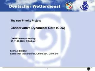
The dynamical core of the COSMO model Besuch des Kurses Geophysical Flows, TU Darmstadt 12. Juli 2018, Offenbach Michael Baldauf Deutscher Wetterdienst, Offenbach M. Baldauf (DWD)
Outlook • Current dynamical core (i.e. for variables u, v, w, p, T) • Runge-Kutta Time Integration scheme • Discretisation of slow process (advection) • Combination with fast processes (sound, buoyancy) • stability • Artificial horizontal diffusion, Smagorinsky-diffusion • Standard idealized test cases M. Baldauf (DWD)
The compressible, non-hydrostatic Euler-equations of the COSMO model in spherical coordinates Qh = diabaticheatproduction Qm = hum. densitychanges in p-eq. additionally: • introduce a hydrostatic, stationary, steady reference state ( p=p0+p', T=T0+T' ) • Transformation to terrain-following coordinates • neglections in pressure equation • shallow/deep atmosphere Namelist-switches:lcori_deep, ladv_deep M. Baldauf (DWD)
Coordinate system • rotated geographical coordinates avoids the ‚pole problem' • Terrain following coordinates • User defined vertical grid stretching: level height z usuallyyousettheselevels in int2lm example: setupof COSMO-DE at DWD level thickness z Grid • structured grid • horizontally and vertically staggered (Arakawa-C, Lorenz) improves dispersion relation of fast waves M. Baldauf (DWD)
Time scales of atmospheric processes Process charact. velocity, ... charact. time type(dx ~ 3 km or dz ~ 30 m) Advection, horiz. 0...10...100 m/s ...300...30 s slow vert. 0...30 m/s ...1 s very fast Sound, horiz. 300 m/s 10 s fast vert. 300 m/s 0.1 s very fast Buoyancy 100 s (=1/N) (slow) Gravity waves, horiz. 0...200 m/s ...15 s fast Coriolis 10000 s (=1/f) slow Diffusion, vert. 0...10...100 m²/s ...100 s ... 10 s fast Sedimentation, vert. ~5 m/s 6 s fast .... Dynamics Physics in compressible, non-hydrostatic models: • vertical processes (sound!) must be treated implicitly • the remaining system is weakly stiff e.g. time-splitting methods M. Baldauf (DWD)
Time integration methods with slow/fast processes • Integration with small time step t (and e.g. additive splitting)inefficient, interest only in slow processes • Semi-implicit method (in combination with Semi-Lagrange-advection)= treat fast process 3D implicit • Time-splitting methodmain reason: fast processes are computationally ‚cheap‘ • Additive splitting (complete operator splitting)but: coupling is too weak (Purser, Leslie, 1991) • partial operator splittingKlemp, Wilhelmson (1978), Wicker, Skamarock (1998, 2002), ... time splitting ratio: ns= T/ t M. Baldauf (DWD)
Time-split Euler-Forward (tsEF) step for a slow/fast process system (partial operator splitting; split-explicit) time splitting ratio: ns= T/ t • apply method of lines (semi-discretization) • costs: 1 Ps, ns Pf • tsEF-scheme not stable (Skamarock, Klemp (1992) MWR, analysis only in time domain) • tsEF-scheme can be stabilized by strong divergence damping (Baldauf (2002) COSMO-Newsl.) • tsEF-scheme can be put into any ODE-solver: • Klemp, Wilhelmson (1978): leapfrog • Wicker, Skamarock (1998): 2-stage Runge-Kutta • Wicker, Skamarock (2002): 3-stage Runge-Kutta dqslow M. Baldauf (DWD)
At first we consider only the slow process (advection) ... M. Baldauf (DWD)
Linear advection equation (1-dim.) discretized: Spatial discretisations of the advection operator (order 1 ... 6) (u>0 assumed) upwind 1st order iadv_order=1 centered diff. 2nd order iadv_order=2 iadv_order=3 iadv_order=4 iadv_order=5 ! iadv_order=6 apart from upwind 1st order, all these schemes are unstable! you need a stable time integration Runge-Kutta Hundsdorfer et al. (1995) JCP Wicker, Skamarock (2002) MWR M. Baldauf (DWD)
q t n+1 n l2tls=.true. irunge_kutta=1 irk_order=2 (not recommended) Time-splitting with Runge-Kutta 2nd order Wicker, Skamarock (1998), MWR RK2-scheme (midpoint-method) for an ODE: dq/dt=f(q) • 2-timelevel scheme • Wicker, Skamarock (1998): upwind-advection stable 3rd order (C<0.88) • combined with time-splitting-idea:‘costs': 2* slow process, 1.5 ns * fast process M. Baldauf (DWD)
q t n+1 n Runge-Kutta Time-Integration autonomous ODE-system (M~108...109...!) explicit N-stage Runge-Kutta-method (to integrate from tn to tn+1): (other equivalent representations are possible) Butcher-Tableau: M. Baldauf (DWD)
Order Conditions for Runge-Kutta (RK) schemes Consistency condition at least 1st order accuracy: example: 4 conditions for RK 3rd order: stage # of ij # of cond. for # of cond. for N N th order RK N th order LC-RK 1 1 1 1 2 3 2 2 3 6 4 3 4 10 8 4 5 15 12(?) 5 ... ... ... ... general theory: Butcher (1964, ...), Butcher (1987) M. Baldauf (DWD)
3-stage RK-Variants: • TVD-RK3 (Shu, Osher, 1988, JCP), RK3b (Hundsdorfer et al., 1995, JCP) irunge_kutta=2 irk_order=3 • RK3a (Hundsdorfer et al., 1995, JCP) • minimal storage scheme (Williamson, 1980, JCP) • Wicker, Skamarock (2002) MWR is not a 3rd order RK-scheme irunge_kutta=1 irk_order=3 (=recommended option!) M. Baldauf (DWD)
Comparison between different numerical schemes for horizontal advection: • Leapfrog + centred diff. 2nd order (C < 1) • Runge-Kutta 2nd order O(dt2) + upwind 3rd order O(dx3) (C < 0.87) • Runge-Kutta 3rd order O(dt3) + upwind 5th order O(dx5) (C < 1.43) dx = 2800m dt = 30 sec. v = 60 m/s C~0.64 Tges=9330 sec. Advection equation: f exakt RK3+up5 Courant number C = v * t / x higher order spatial discretization better represents the solution if the fields are well resolved Leapfrog RK2+up3 grid point M. Baldauf (DWD)
Stable Courant-numbers for advection schemes Courant number C = v * t / x up1 cd2 up3 cd4 up5 cd6 Leapfrog 0 1 0 0.72 0 0.62 LC-RK1 (Euler) 1 0 0 0 0 0 LC-RK2 1 0 0.874 0 0 0 LC-RK3 1.256 1.732 1.626 1.262 1.435 1.092 LC-RK4 1.393 2.828 1.745 2.061 1.732 1.783 LC-RK5 1.609 0 1.953 0 1.644 0 LC-RK6 1.777 0 2.310 0 1.867 0 LC-RK7 1.977 1.764 2.586 1.286 2.261 1.113 Wicker, Skamarock (2002) MWR: Leapfrog, RK2, RK3, Baldauf (2008) JCP M. Baldauf (DWD)
Stability limit for the ‚effective Courant-number‘ for advection schemes Ceff := C / s, s = stage of RK-scheme up1 cd2 up3 cd4 up5 cd6 Euler 1 0 0 0 0 0 LC-RK2 0.5 0 0.437 0 0 0 LC-RK3 0.419 0.577 0.542 0.421 0.478 0.364 LC-RK4 0.348 0.707 0.436 0.515 0.433 0.446 LC-RK5 0.322 0 0.391 0 0.329 0 LC-RK6 0.296 0 0.385 0 0.311 0 LC-RK7 0.282 0.252 0.369 0.184 0.323 0.159 Baldauf (2008) JCP: general stability theory about LC-RK schemes (in particular for advection operators) M. Baldauf (DWD)
2D-advection in RK-schemes by a simple adding of tendencies(operator splitting (e.g. corner transport upstream (CTU) method) is not possible for upstream 3., 5., ... order ) this is limited by |Cx| + |Cy| < Ccrit,1D(Baldauf (2008) JCP) 2-dim. horizontal Advection Subr. check_cfl_horiz_advection Vertical Advection centered differences 2nd order; implicit ( in particular in convection-resolving simulations, the vertical Courant numbers can heavily exceed 1!) solve a tri-diagonal linear equation system y_vert_adv_dyn=„impl2“ (alternatives: „impl3“, „expl“) M. Baldauf (DWD)
The overalltime stepdtof COSMO is in factdeterminedby theadvection Courant number. Ifwerequirethat COSMO shouldbestableforvhor < 160 m/s (either in x- or in y-direction) thenthefollowingvaluesarerecommended (for 5th orderadvectionandthe RK3 scheme Cmax=1.43): M. Baldauf (DWD)
Now we combine slow and fast processes ... M. Baldauf (DWD)
COSMO equations, simplifiedfor a • 2D (x-z-) slice model • without Coriolis force • on a flat plane • dry atmosphere fast waves hydrostatic reference state (p0, T0), p=p0+p’ T=T0+T’ M. Baldauf (DWD)
Forward-Backward schemefor the horizontal fast waves part example: 1D wave equation phase velocity: Forward-backward scheme (Mesinger, 1977): (timestep n, grid position j, on a staggered grid) forward step backward step This scheme is stable for ct / x< 1. (remark: an explicit scheme is completely unstable!) M. Baldauf (DWD)
Discretized and linearized 2D slice model, fast waves part artificial divergence damping sound waves buoyancy oscillations x, z,: centered difference derivatives Sound waves alone: stable for βs ≥ ½ and Cx := csndt/x < 1, no constraint for Cz !Buoyancy oscill. alone: unconditionally stable for βb ≥ ½ M. Baldauf (DWD)
kxx = -..+, kzz = -..+ Von-Neumann stability analysis Linearize PDE-system for u(x,z,t), w(x,z,t), ... with constant coefficients Discretization unjl, wnjl, ... (grid sizes x, z) single Fourier-Mode: unjl= un(kx, kz) exp( i (kx j x + kz l z) ) 2-timelevel schemes: Determine eigenvalues iof 4x4 amplification-matrix Q(kx, kz) scheme is stable, if maxi |i| 1 find i analytically or numerically by scanning Restrictions: • no boundaries (wave expansion in extended medium) • base state: p0=const, T0=const (for the coefficients) (but stratification dT0/dz 0 possible) only applicable to vertical wavelengths << 10 km • no vertical grid stretching • no orography (i.e. no metric terms) • only horizontal advection Baldauf (2010) MWR
Stability of single waves for advection + sound (partial operator splitting with RK3, Cadv=1.0, Csnd,x=0.6) (without divergence damping) Sound term discretization: Spatial: centered differences Temporal: Forward-backward (Mesinger, 1977) Vertically implicit (βs ≥ ½) • stable for Csnd,x < 1, Csnd,z arbitrary but in combination with (slow) advection: even for βs >½ (‚off-centering‘), a slight instability of horizontal waves occurs βs=0.5 kzz βs=0.7 kxx M. Baldauf (DWD)
Divergence damping leads to a diffusion of divergence damping of sound waves Isotropic div. damping recommended: Gassmann, Herzog (2007) MWR Courant-numbers: 2D, explicit, stagg. grid: stable for Cdiv,x + Cdiv,z < ½ 2D, hor. expl.-vert. impl., stagg. grid: stable for Cdiv,x < ½, Cdiv,z arbitrary Cdiv,x = 0.1 for COSMO-DE div=160000 m²/s div / (cs2t )~ 0.3 Skamarock, Klemp (1992) MWR, Wicker, Skamarock (2002) MWR M. Baldauf (DWD)
Stability of single waves for advection + sound (partial operator splitting with RK3, Cadv=1.0, Csnd,x=0.6) without div.-damping with div.-damping βs=0.5 kzz βs=0.7 kxx M. Baldauf (DWD)
Artificial horizontal diffusion 4th order dim.-less diffusion coeff.: 4 := K4t / x4 stable + 'non-oszillating' sinus-waves for 0 4 1/64 0.016 (for Leapfrog (2t !): 0 4 1/128) in COSMO-EU: 4 = 0.25 / (24) 0.0013; used only for u,v,w in COSMO-DE: 4 = 0.1 / (24) 0.0005; used only for u,v,w • Diffusion 4th order is not monotone! flux limitation (Doms, 2001) • additional orography-limitation: diffus. flux=0, if slope of a coordinate plane > 250 m / x Amplification factor for 4 0.001 k * dx Namelist-Param.: hd_corr_u_in, hd_corr_u_bd, hd_corr_t_in, ... M. Baldauf (DWD)
COSMO-DE at 26.08.2011, 6 UTC run M. Baldauf (DWD)
Additionally a non-linear Smagorinsky-diffusion is needed Smagorinsky (1963) MWR: • Smagorinsky diffusion is able to avoid shear instabilities • Synop-Verification of COSMO-DE experiments show, that the impact on the forecast quality is small(in particular for summerly convection)the value of the Smagorinsky-coeff. cS=0.03 is chosen quite low towards the 'standard' value of cS~0.1 • the additional computational costs are ~1% • was introduced in COSMO 4.21 • Lit.: Baldauf, Zängl (2012) COSMO-Newsletter ls= cs l(x, y) dimensionless diffusion coefficient: ksmag := Ksmag * t / ls2 stability ksmag < ½ l_Smag_diff=.TRUE. M. Baldauf (DWD)
Kinetic energy spectrum k-3 Calculation of spectra in x direction. Averaging of ~400 such spectra k-5/3 effective resolution ~ 6 dx (Abb. KE-Spektrum ) without with artificial horizontal 4th order and Smagorinsky-diffusion Skamarock (2003) MWR M. Baldauf (DWD)
Standard idealized test cases for non-hydrostatic models M. Baldauf (DWD)
Test case 4.1: 2D linear flow over mountains setup: Schär et al. (2002) Orography: h0=25m, b=5km, =4km Frh=40, Fra=0.1 … 0.5 u0=10m/s, N=0.01 1/s, T(z=0)=288K comparewithanalytic linear solution: Baldauf, 2008, COSMO-NL (usesonly a fewfurtherapproximations, e.g. itis a fullycompressiblesolution) • Test properties: • test dry Euler equationswithout Coriolis terms • stationary • withorography test also metricterms • smallamplitude linear comparisonwithanalyticsolutionpossible M. Baldauf (DWD)
Test case 4.1: 2D linear flow over mountains x=500m z=300m COSMO ICON colorsandblackdottedlines: COSMO or ICON greylines:analyticsolution vertically equidistant grid M. Baldauf (DWD)
Test case 4.1: 2D linear flow over mountains x=250m z=150m COSMO ICON colorsandblackdottedlines: COSMO or ICON greylines:analyticsolution vertically equidistant grid M. Baldauf (DWD)
Test case 4.3a: 3D linear flow over mountains vertically stretched grid: zbottom = 24.7m ztop = 976 m h0=1 m, a=5000m u0=20 m/s N=0.01 1/s Frh=2000, Fra =0.4 x=500m M. Baldauf (DWD)
Test case 4.3a: 3D linear flow over mountains colorsandgreylines: COSMO simulation blacklines:analyticsolution M. Baldauf (DWD)
Linear, unsteady gravity wave Skamarock, Klemp (1994) MWR Baldauf, Brdar (2013) QJRMS M. Baldauf (DWD)
Initialization similar to Skamarock, Klemp (1994) Small scale test with a basic flow U0=20 m/s f=0 Black lines: analytic solution (Baldauf, Brdar (2013) QJRMS) Shaded: COSMO M. Baldauf (DWD)
Large scale test without advection but with Coriolis force colors and black dotted lines: ICON, blue lines: analytic solution dx=10km dx=2.5km M. Baldauf (DWD)
Test of the dynamical core: density current (Straka et al., 1993)
COSMO at t=15 min. for x= 200, 100, 50, 25m a cold bubble (centered around x=25.6km, z=3 km) falls down and develops a gust front(Kelvin-Helmholtz instabilities) Reference solution from Straka et al. (1993): M. Baldauf (DWD)
Physics-Dynamics-coupling fields n=(u, v, w, pp, T, ...)n Physics (I) • Radiation • Convection • Coriolis force ('old' scheme) • Turbulence ‚Physics (I)‘-tendencies n(phys I) Dynamics Runge-Kutta [(phys) +(adv) --> fast_waves ] fields *=(u, v, w, pp, T, ...)* Physics (II) • Cloud Physics fields n+1=(u, v, w, pp, T, ...)n+1 M. Baldauf (DWD)
Other numerical stuff not mentioned here: • New reference state • Tracer advection • boundary conditions • bottom (physical) BC's • lateral BC's • upper BC's M. Baldauf (DWD)
Thank you for your attention ! A Description of the Nonhydrostatic Regional COSMO-Model: G. Doms, M. Baldauf: Part I: Dynamics and Numerics U. Schättler, G. Doms, C. Schraff: Part VI: Users Guide http://www.cosmo-model.org/content/model/documentation/core/default.htm M. Baldauf (DWD)