Macroeconometric Models
Macroeconometric Models. Simultaneous Equations Vector Auto Regression Forecasting. A simple Example of the Simultaneous Equation System. General Form for the Simultaneous Equation System. ………………………………………………………………. Impact and Shock Analysis in a Simultaneous Equation System. .

Macroeconometric Models
E N D
Presentation Transcript
Macroeconometric Models Simultaneous Equations Vector Auto Regression Forecasting
General Form for the Simultaneous Equation System ………………………………………………………………
Impact and Shock Analysis in a Simultaneous Equation System .
Checking Rank Identification Condition for the above System Consumption function: It is obvious that there exists at least on non-singular matrix of order M-1. Tax function:
Checking Rank Identification Condition for the above System Import Interest Rate Investment
Some Techniques for Estimation of the Simultaneous Equations System
Estimation of Simultaneous System using PcGive C = + 0.2128*M4 + 1.407*G + 0.1767*X + 8.059e+004 (SE) (0.0266) (0.212) (0.154) (1.63e+004) Y = + 0.2617*M4 + 2.86*G + 1.348*X + 8.862e+004 (SE) (0.0454) (0.361) (0.262) (2.78e+004) T = + 0.3204*M4 + 0.9521*G - 0.08909*X - 7.533e+004 (SE) (0.02) (0.159) (0.116) (1.23e+004) M = + 0.06508*M4 - 0.4738*G + 1.003*X + 4.34e+004 (SE) (0.0198) (0.157) (0.114) (1.21e+004) r = - 2.384e-005*M4 + 0.0001148*G + 6.273e-005*X - 7.408 (SE) (6.2e-006) (4.93e-005) (3.58e-005) (3.79) I = + 0.02907*M4 + 0.0684*G + 0.2681*X + 4.292e+004 (SE) (0.0229) (0.182) (0.132) (1.4e+004)
References • Bhattarai (2004) REVIEW OF MACROECONOMETRIC MODELS FOR ANALYSIS AND FORECASTING, University of Hull. • Burns, A and W. Michell, (1946), “Measuring Business Cycles” NBER, New York. • Campbell J. Y. and R.J. Shiller (1987) Cointegration and Tests of Present Value Models, Journal of Political Economy, 95, 5, pp. 1062-1087. • Doornik J.A and D.F. Hendry (2003) Econometric Modelling Using PCGive Volumes I, II and II, Timberlake Consultant Ltd, London. • Garratt A., K. Lee, M.H. Pesaran and Y. Shin (2003) A Structural Cointegration VAR Approach to Macroeconometric Modelling, Economic Journal. • Hendry D.F. (1997) Dynamic Econometrics, Oxford University Press. • Harris R. and R. Sollis (2003) Applied Time Series Modelling and Forecasting, John Willey. • Holly S and M Weale Eds.(2000) Econometric Modelling: Techniques and Applications, pp.69-93, the Cambridge University Press. • Johansen Soren (1988) Estimation and Hypothesis Testing of Cointegration Verctors in Gaussian Vector Autoregressive Models, Econometrica, 59:6, 1551-1580. • Koopman SJ, AC Harvey, JA Doornik and N. Shephard (2000) Structural Time Series Analyser, Modeller and Predictor (STAMP), Timberlake Consultants Ltd. • Pagan A. and M. Wickens (1989) A Survey of Some Recent Econometric Methods, Economic Journal, 99 pp. 962-1025. • Wallis KF. (1989) Macroeconomic Forecasting: A Survey, Economic Journal, 99, March, pp 28-61.
A Sample Batch Code for PC-Give • //Batch code for the final specification: • module("PcGive"); • package("PcGive"); • usedata("Macrotimeseries-UK.xls"); • system • { • Y = C, Y, T, M; • Z = C_1, Y_1, T_1, M_1, G, G_1, M4, M4_1; • U = Constant; • } • model • { • C = C_1, Y_1, T_1, M_1, G, G_1, M4, M4_1; • Y = C_1, Y_1, T_1, M_1, G, G_1, M4, M4_1; • T = C_1, Y_1, T_1, M_1, G, G_1, M4, M4_1; • M = C_1, Y_1, T_1, M_1, G, G_1, M4, M4_1; • } • estimate("FIML", 1961, 1, 2001, 1);