Download
1 / 56
560 likes | 579 Views
Investigating low-frequency seismicity using Viscoelastic finite-difference model & Coda Q analysis, focusing on amplitude losses in volcanic environments. Discussing conduit resonance, energy propagation, and source trigger mechanisms. Illustrating the importance of low-frequency earthquakes in eruption prediction and magma processes.

E N D
Low frequency coda decay: separating the different components of amplitude loss. Patrick Smith Supervisor: Jürgen Neuberg School of Earth and Environment, The University of Leeds.
Outline of Presentation • Background: low-frequency seismicity, project context, quantifying amplitude losses • Methodology: Viscoelastic finite-difference model & Coda Q analysis • Results and Implications: plus some discussion of future work
High frequency onset • Coda: • harmonic, slowly decaying • low frequencies (0-5 Hz) Low frequency seismicity What are low-frequency earthquakes? Specific to volcanic environments →Are a result of interface waves originating at the boundary between solid rock and fluid magma
Conduit Resonance Propagation of seismic energy • Energy travels as interface waves along conduit walls at velocity controlled by magma properties • Top and bottom of the conduit act as reflectors and secondary sources of seismic waves • Fundamentally different process from harmonic standing waves in the conduit Source Trigger Mechanism = Brittle Failure of Melt
Propagation of seismic energy ESC 2007 S-wave P-wave
Propagation of seismic energy ESC 2007 Interface waves S-wave P-wave
Propagation of seismic energy ESC 2007 Interface waves
Propagation of seismic energy ESC 2007 Interface waves
Propagation of seismic energy ESC 2007 Interface waves
Propagation of seismic energy ESC 2007 Interface waves
Propagation of seismic energy ESC 2007
Propagation of seismic energy ESC 2007 reflections
Propagation of seismic energy ESC 2007 reflections
Propagation of seismic energy ESC 2007
Propagation of seismic energy Acoustic velocity of fluid ESC 2007 FAST MODE: I1 NORMAL DISPERSION Low frequencies High frequencies High frequencies SLOW MODE: I2 INVERSE DISPERSION Low frequencies
Propagation of seismic energy ESC 2007 I1 I2
Propagation of seismic energy ESC 2007 I1 S I2
Propagation of seismic energy ESC 2007 I1 S I2
Propagation of seismic energy ESC 2007 I1 S I2
Propagation of seismic energy ESC 2007 I2 ‘Secondary source’
Propagation of seismic energy ESC 2007 Surface-wave ‘Secondary source’
Propagation of seismic energy ESC 2007 Surface-wave
Propagation of seismic energy ESC 2007 I1R1
Propagation of seismic energy ESC 2007 I1R1
Propagation of seismic energy ESC 2007 I1R1 I2
Propagation of seismic energy ESC 2007 I2 ‘Secondary source’
Propagation of seismic energy ESC 2007 ‘Secondary source’
Propagation of seismic energy ESC 2007
Propagation of seismic energy ESC 2007
Propagation of seismic energy ESC 2007
Propagation of seismic energy ESC 2007 Most of energy stays within the conduit
Propagation of seismic energy ESC 2007 Most of energy stays within the conduit
Propagation of seismic energy ESC 2007 Most of energy stays within the conduit
Propagation of seismic energy ESC 2007 Most of energy stays within the conduit
Propagation of seismic energy ESC 2007
Propagation of seismic energy ESC 2007 R2
Propagation of seismic energy ESC 2007 Events are recorded by seismometers as surface waves R2
Why are low frequency earthquakes important? • Have preceded most major eruptions in the past • Correlated with the deformation and tilt - implies a close relationship with pressurisation processes (Green & Neuberg, 2006) • One of the few tools that provide direct link between surface observations and internal magma processes
Attenuation via Q Properties of the magma Conduit geometry + Context: combining magma flow modelling & seismicity Conduit Properties Seismic parameters Signal characteristics Magma properties (internal) seismic signals (surface)
gas loss plug flow slip slip . 7 e m > 10 Pa depth of brittle failure parabolic flow Stress threshold: Seismic trigger mechanism Collier & Neuberg, 2006; Neuberg et al., 2006
Swarms preceding dome collapse Swarm structure Increased event rates Similar earthquake waveforms Linked to magma extrusion
V m/s Towards a Magma Flow Meter Photo : R Herd, MVO
Seismic attenuation in magma amplitude decay true damping Why is attenuation important? • Needed to quantitatively link source and surface amplitudes. • Allows us to link signal characteristics, e.g. amplitude decay of the coda, to properties of the magma such as the viscosity Definitions: Radiative (parameter contrast) Intrinsic (anelastic) Apparent (coda) (Aki, 1984)
Quantifying amplitude losses Intrinsic attenuation in magma causes some damping of signal amplitude – but how much? Further amplitude loss due to geometric spreading – signal travels to seismometer as surface wave: but DOES NOT contribute to apparent Q ! rs rf af as Q-1 Seismometer Qr-1 T (transmission coefficient) R (reflection coefficient) Qi Contrast in elastic parameters causes some energy to be transmitted and some to be reflected Total amplitude decay is a combination of these contributions: Q-1=Qi-1+Qr-1 Trigger mechanism: brittle failure at conduit walls
Amplitude decay of coda Comparison of approaches: • Kumagai & Chouet: used complex frequencies to derive apparent Q from signals → resonating crack finite-difference model using bubbly water mixture to reproduce signals. ONLY radiative Q – no account of intrinsic Q • Our approach – viscoelastic finite-difference model, with depth dependent parameters: includes both intrinsic attenuation of magma and radiative energy loss due to elastic parameter contrast. Figure from Kumagai & Chouet (1999)
Modelling Intrinsic Q BGA 2007 Intrinsic Q is dependent on the properties of the magma: Viscosity (of melt & magma) Gas content Diffusivity • To include anelastic ‘intrinsic’ attenuation – the finite-difference code uses a viscoelastic medium: stress depends on both strain and strain rate. • Parameterize material using Standard Linear Solid (SLS): viscoelastic rheological model • whose mechanical analogue is as shown: Use in finite-difference code to model intrinsic Q
Finite-Difference Method ESC WG 2007 Free surface • 2-D O(Δt2,Δx4) scheme based on Jousset, Neuberg & Jolly (2004) • Volcanic conduit modelled as a viscoelastic fluid-filled body embedded in homogenous elastic medium Solid medium (elastic) Seismometers ρ = 2600 kgm-3 α = 3000 ms-1 β = 1725 ms-1 Source Signal: 1Hz Küpper wavelet (explosive source) Fluid magma (viscoelastic) Variable Q Damped Zone Domain Boundary
Determining apparent (coda) Q A0 A1 A2 A3 Amplitude 0 Synthetic trace -A0 1 2 3 4 0 Time [number of cycles] p A2 p 1 - Q = = Q A2 A1 – A2 (taken from Chouet 1996) Model produces harmonic, monochromatic synthetic signals Coda Q methodology: Aki & Richards (2003) • Decays by factor (1p/Q) each cycle Take ratio of successive peaks, e.g. A1
Calculation of coda Q Apparent Q value based on envelope maxima -22.6 Linear Fit Data -22.8 Unfiltered data -23 -23.2 log(Amplitude) -23.4 -23.6 Gradient of line =-0.10496 -23.8 Q value from gradient = 31.5287 -24 0 2 4 6 8 10 12 Time [cycles] Calculating Q using logarithms Gradient of the line given by: Hence Q is given by: