Cross-Sectional Properties of Coronal Loops

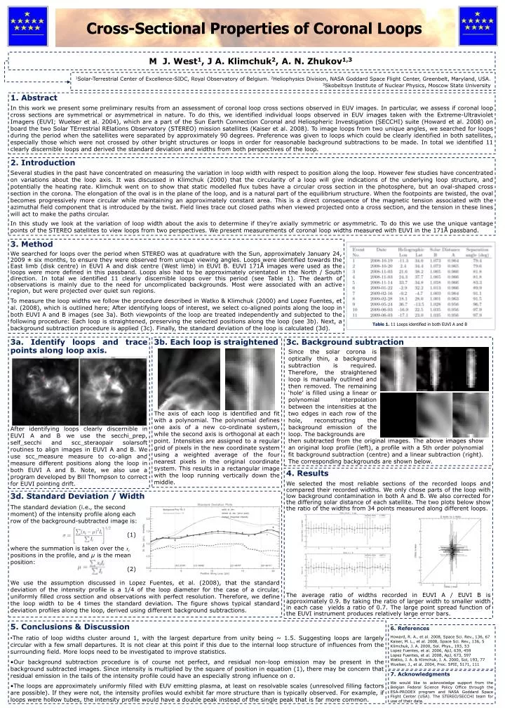
1. Table 1.11 Loops identified in both EUVI A and B 3a. Identify loops and trace points along loop axis. After identifying loops clearly discernible in EUVI A and B we use the secchi_prep, self_secchi and scc_steraopair solarsoft routines to align images in EUVI A and B. We use scc_measure measure to co-align and measure different positions along the loop in both EUVI A and B. Note, we also use a program developed by Bill Thompson to correct for EUVI pointing drift. 3b. Each loop is straightened The axis of each loop is identified and fit with a polynomial. The polynomial defines one axis of a new co-ordinate system, while the second axis is orthogonal at each point. Intensities are assigned to a regular grid of pixels in the new coordinate system using a weighted average of the four nearest pixels in the original coordinate system. This results in a rectangular image with the loop running vertically down the middle. 3c. Background subtraction Since the solar corona is optically thin, a background subtraction is required. Therefore, the straightened loop is manually outlined and then removed. The remaining ‘hole’ is filled using a linear or polynomial interpolation between the intensities at the two edges in each row of the hole, reconstructing the background emission of the loop. The backgrounds are then subtracted from the original images. The above images show an original loop profile (left), a profile with a 5th order polynomial fit background subtraction (centre) and a linear subtraction (right). The corresponding backgrounds are shown below. 4. Results We selected the most reliable sections of the recorded loops and compared their recorded widths. We only chose parts of the loop with low background contamination in both A and B. We also corrected for the differing solar distance of each satellite. The two plots below show the ratio of the widths from 34 points measured along different loops. The average ratio of widths recorded in EUVI A / EUVI B is approximately 0.9. By taking the ratio of larger width to smaller width in each case yields a ratio of 0.7. The large point spread function of the EUVI instrument produces relatively large error bars. 3d. Standard Deviation / Width The standard deviation (i.e., the second moment) of the intensity profile along each row of the background-subtracted image is: (1) where the summation is taken over thexi positions in the profile, and μ is the mean position: (2) We use the assumption discussed in Lopez Fuentes, et al. (2008), that the standard deviation of the intensity profile is a 1/4 of the loop diameter for the case of a circular, uniformly filled cross section and observations with perfect resolution. Therefore, we define the loop width to be 4 times the standard deviation. The figure shows typical standard deviation profiles along the loop, derived using different background subtractions. Cross-Sectional Properties of Coronal Loops M J. West1, J A. Klimchuk2, A. N. Zhukov1,3 1Solar-Terrestrial Center of Excellence-SIDC, Royal Observatory of Belgium. 2Heliophysics Division, NASA Goddard Space Flight Center, Greenbelt, Maryland, USA. 3Skobeltsyn Institute of Nuclear Physics, Moscow State University 1. Abstract In this work we present some preliminary results from an assessment of coronal loop cross sections observed in EUV images. In particular, we assess if coronal loop cross sections are symmetrical or asymmetrical in nature. To do this, we identified individual loops observed in EUV images taken with the Extreme-Ultraviolet Imagers (EUVI; Wuelser et al. 2004), which are a part of the Sun Earth Connection Coronal and Heliospheric Investigation (SECCHI) suite (Howard et al. 2008) on board the two Solar TErrestrial RElations Observatory (STEREO) mission satellites (Kaiser et al. 2008). To image loops from two unique angles, we searched for loops during the period when the satellites were separated by approximately 90 degrees. Preference was given to loops which could be clearly identified in both satellites, especially those which were not crossed by other bright structures or loops in order for reasonable background subtractions to be made. In total we identified 11 clearly discernible loops and derived the standard deviation and widths from both perspectives of the loop. 2. Introduction Several studies in the past have concentrated on measuring the variation in loop width with respect to position along the loop. However few studies have concentrated on variations about the loop axis. It was discussed in Klimchuk (2000) that the circularity of a loop will give indications of the underlying loop structure, and potentially the heating rate. Klimchuk went on to show that static modelled flux tubes have a circular cross section in the photosphere, but an oval-shaped cross section in the corona. The elongation of the oval is in the plane of the loop, and is a natural part of the equilibrium structure. When the footpoints are twisted, the oval becomes progressively more circular while maintaining an approximately constant area. This is a direct consequence of the magnetic tension associated with the azimuthal field component that is introduced by the twist. Field lines trace out closed paths when viewed projected onto a cross section, and the tension in these lines will act to make the paths circular. In this study we look at the variation of loop width about the axis to determine if they’re axially symmetric or asymmetric. To do this we use the unique vantage points of the STEREO satellites to view loops from two perspectives. We present measurements of coronal loop widths measured with EUVI in the 171Å passband. 3. Method We searched for loops over the period when STEREO was at quadrature with the Sun, approximately January 24, 2009 ± six months, to ensure they were observed from unique viewing angles. Loops were identified towards the East limb (disk centre) in EUVI A and disk centre (West limb) in EUVI B. EUVI 171Å images were used as the loops were more defined in this passband. Loops also had to be approximately orientated in the North / South direction. In total we identified 11 clearly discernible loops over this period (see Table 1). The dearth of observations is mainly due to the need for uncomplicated backgrounds. Most were associated with an active region, but were projected over quiet sun regions. To measure the loop widths we follow the procedure described in Watko & Klimchuk (2000) and Lopez Fuentes, et al. (2008), which is outlined here; After identifying loops of interest, we select co-aligned points along the loop in both EUVI A and B images (see 3a). Both viewpoints of the loop are treated independently and subjected to the following procedure: Each loop is straightened, preserving the selected positions along the loop (see 3b). Next, a background subtraction procedure is applied (3c). Finally, the standard deviation of the loop is calculated (3d). • 5. Conclusions & Discussion • The ratio of loop widths cluster around 1, with the largest departure from unity being ~ 1.5. Suggesting loops are largely circular with a few small departures. It is not clear at this point if this due to the internal loop structure of influences from the surrounding field. More loops need to be investigated to improve statistics. • Our background subtraction procedure is of course not perfect, and residual non-loop emission may be present in the background subtracted images. Since intensity is multiplied by the square of position in equation (1), there may be concern that residual emission in the tails of the intensity profile could have an especially strong influence on σ. • The loops are approximately uniformly filled with EUV emitting plasma, at least on resolvable scales (unresolved filling factors are possible). If they were not, the intensity profiles would exhibit far more structure than is typically observed. For example, if loops were hollow tubes, the intensity profile would have a double peak instead of the single peak that is far more common. 6. References Howard, R. A., et al. 2008, Space Sci. Rev., 136, 67 Kaiser, M. L., et al. 2008, Space Sci. Rev., 136, 5 Klimchuk, J. A. 2000, Sol. Phys., 193, 53 Lopez Fuentes, et al. 2006, ApJ, 639, 459 Lopez Fuentes, et al. 2008, ApJ, 673, 597 Watko, J. A. & Klimchuk, J. A. 2000, Sol, 193, 77 Wuelser, J., et al. 2004, Proc. SPIE, 5171, 111 7. Acknowledgments We would like to acknowledge support from the Belgian Federal Science Policy Office through the ESA-PRODEX program and NASA Goddard Space Flight Center (USA). The STEREO/SECCHI team for use of their data.