Download
1 / 31
310 likes | 513 Views
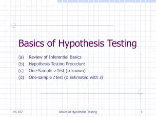
Basics of Hypothesis Testing. Review of Inferential Basics Hypothesis Testing Procedure One-Sample z Test ( σ known) One-sample t test ( σ estimated with s ). Review of Some Basics. Population all possible values Sample a portion of the population

E N D
Basics of Hypothesis Testing Review of Inferential Basics Hypothesis Testing Procedure One-Sample z Test (σ known) One-sample t test (σ estimated with s) Basics of Hypothesis Testing
Review of Some Basics • Population all possible values • Sample a portion of the population • Statistical inference generalizing from a sample to a population with calculated degree of certainty • Two forms of statistical inference • Estimation • Hypothesis testing • Parameter a numerical characteristic of a population, e.g., population mean µ, population standard deviation σ • Statistic a numerical characteristic calculated in the sample, e.g., sample mean x-bar, sample standard deviation s Basics of Hypothesis Testing
Recall the distinction between parameters and statistics Basics of Hypothesis Testing
Recall how sample means (xbars) vary The sampling distribution of the mean (SDM) tends to be Normal with mean µ and a standard deviation called the SE Basics of Hypothesis Testing
Hypothesis Testing Procedure • A. Hypotheses • B. Test Statistic • C. P-value • D. Significance level (optional) Basics of Hypothesis Testing
Step A. Hypotheses • Take the research question and convert it to statistical hypotheses • State statistical hypotheses in null and alternative forms • H0 Null hypothesis “no difference in the population” • Ha Alternative hypothesis “difference in the population” • Seek evidence against H0 as a way of bolstering H1 Basics of Hypothesis Testing
Step B. Test Statistic • Calculate the appropriate test statistic • There are many types of test statistics, depending on the conditions of the data • This Chapter introduces this particular one-sample z statistic: Basics of Hypothesis Testing
Step C. P-value • Convert zstat to P-value using table or software • The P-value is the AUC in the tail of the SDM beyond the test statistics. • The P-value answer the question: What is the probability of the observed test statistics or one that is more extreme assuming H0 is true? • Small P-value good evidence against H0 • Although it unwise to draw too-firm cutoffs, here are guidelines for the beginner: • P > 0.10 evidence against H0not significant • 0.05 < P 0.10 evidence against H0marginally significant • 0.01 < P 0.05 evidence against H0significant • P 0.01 evidence against H0highly significant Smaller and smaller P-values provide stronger and stronger evidence against Basics of Hypothesis Testing
Step D. Significance level (optional) • Declare acceptable false rejection (Type I) error rate α • α can be set at any level (e.g., 1 in 20, 1 in 50, 1 in 100) • When P <α reject H0 at α level of significance Basics of Hypothesis Testing
Illustrative Example: Lake Wobegon, Study Design • Research question: Does a particular population of children have higher than average intelligence scores? • Study design • Weschler intelligence scores are Normal with µ = 100 and s = 15 • Take a SRS • Measure WIS {116, 128, 125, 119, 89, 99, 105, 116, 118} • Calculate sample mean: x-bar = 112.8 • Ask: Does this provide sufficient evidence that population mean (μ) is greater than expected (100)? Basics of Hypothesis Testing
Illustrative Example: Lake Wobegon, Step A • Under the null hypothesis of “no difference” H0: µ = 100 • Under the alternative hypothesis of “difference” Ha: µ > 100 Note: (a) Hypotheses address the parameter (not the statistic) (b) The value of the parameter under H0 is based on the research question (NOT the data) Basics of Hypothesis Testing
Illustrative Example: Lake Wobegon, Step B • The test statistics for this problem is the one-sample z statistic • This statistic assumes H0 is correct • It then standardizes the sample mean (i.e., turns it into a z-score): Basics of Hypothesis Testing
Illustrative Example: Lake Wobegon, Step C • The test statistic is converted to a P-value • Assuming H0 true, where does zstat fall on the curve? • P value area under curve beyond zstat • Use Z table (or software) to find Pr(Z≥ zstat) = Pr(Z≥ 2.56) = 0.0052 • The P-value of 0.0052 provides strong (“highly significant”) evidence against H0 Basics of Hypothesis Testing
Illustrative Example: Lake Wobegon Step D (Optional) P = 0.0052 is highly significant evidence against H0 The smaller the P, the more significant the evidence. See guidelines in earlier slide. Basics of Hypothesis Testing
The one-sided alternative • The prior test made a supposition about the direction of the difference • The test had a “one-sided H1” We looked only at one side of the SDM Basics of Hypothesis Testing
The two-sided alternative • Allows for unanticipated findings either up or down from expected • The requires a two-sided test • The two-sided test looks at both tails • Just double the one-sided P • Lake Wobegon example two-sided P = 2 × 0.0052 = 0.0104 Basics of Hypothesis Testing
Illustrative example: “Anemia” • Research question: A public health official suspects a particular population is anemic • Hemoglobin is a protein in red blood cells that carries oxygen • People with less than 12 g/dl hemoglobin are anemic • We know that hemoglobin levels in children are Normal with standard deviation σ = 1.6 g/dl • Data: The researcher measures hemoglobin in 50 children and finds x-bar = 11.3 Basics of Hypothesis Testing
Step A: Anemia example • We seek evidence against µ = 12. Thus, H0: µ = 12 • The one-sided alternative is H1: µ < 12 • The two-sided alternative is H1: µ 12 • Let’s do a two-sided test (much more common in practice) Basics of Hypothesis Testing
Step B: Test statistic Basics of Hypothesis Testing
Step C. P-value • Pr(Z < -3.10) = 0.0010 • Double this b/c the alternative is two-sided: P = 2 × 0.0010 = 0.0020 • Comment: Under H0, xbar~N(12, 0.226), I’ll draw this on the board so you see that an x-bar of 11.3 is in the far left tail Basics of Hypothesis Testing
Step D: Conclusion P = 0.0020 evidence against H0 is highly significant Basics of Hypothesis Testing
Conditions necessary for z test • Simple random sample (SRS) • Normal population or large sample • sknown (not calculated) What do you do when σis not known? Use a t procedure! Basics of Hypothesis Testing
Diabetic weight illustrative example • Claim: “diabetics are over-weight” • Data are “% of ideal body weight” • n = 18 • Sample mean (x-bar) = 112.778 • Sample standard deviation (s) = 14.424 Basics of Hypothesis Testing
Step A: Hypotheses (diabetic weight) • Research claim is “diabetics are over-weight” • Convert claim to a null hypothesis • “Diabetics are not overweight” • Not overweight = 100 of ideal body weight • Therefore, H0: µ = 100 • Alternative hypothesis can be • H1: µ 100 (two-sided) • H1: µ > 100 (one-sided to right) • H1: µ < 100 (one-sided to left) Basics of Hypothesis Testing
Step B: Test statistic tstat tells you how many standard errors the sample mean falls from hypothesized population mean Basics of Hypothesis Testing
Step C: P value (Diabetic weight) • t table: wedge tstat between t landmarks • Example: tstat = 3.76 on t with 17 df falls between 3.646 (right tail 0.001) and 3.965 (right tail 0.0005) • Two-tailed P is twice the one-tailed values: P less than 0.002 and more than 0.001 • P = 0.0016 (via software) Basics of Hypothesis Testing
Step D: Conclusion P = 0.0016 provides highly significant evidence against H0 Basics of Hypothesis Testing
Consequences of test decisions Probability (type I error) = a Probability (type II error) = b Basics of Hypothesis Testing
Type II errors (β) • We have considered only type I (a) errors • In the next chapter we will take up the issue of type II (b) errors • b = Pr(rejecting a false H0) • The complement of b is 1 – b = ”Power” Basics of Hypothesis Testing
Fallacies of hypothesis testing • Failure to reject H0 = acceptance of H0 (WRONG!) • P value = probability H0 is incorrect (WRONG!) • Statistical significance implies biological or social importance (WRONG!) Basics of Hypothesis Testing
Beware! Hypothesis testing addresses random error only. It does not account for many problems encountered in practice, such as measurement error and sampling biases Basics of Hypothesis Testing