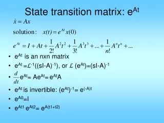
State transition matrix: e At
State transition matrix: e At. e At is an nxn matrix e At = ℒ -1 ((sI-A) -1 ), or ℒ (e At )=(sI-A) -1 e At = Ae At = e At A e At is invertible: (e At ) -1 = e (-A)t e A0 =I e At1 e At2 = e A(t1+t2). I/O model to state space. Controller canonical form is not unique

State transition matrix: e At
E N D
Presentation Transcript
State transition matrix: eAt • eAt is an nxn matrix • eAt =ℒ-1((sI-A)-1), or ℒ (eAt)=(sI-A)-1 • eAt= AeAt=eAtA • eAt is invertible: (eAt)-1= e(-A)t • eA0=I • eAt1 eAt2= eA(t1+t2)
I/O model to state space • Controller canonical form is not unique • This is also controller canonical form
Solution of state space model Recall: sX(s)-x(0)=AX(s)+BU(s) (sI-A)X(s)=BU(s)+x(0) X(s)=(sI-A)-1BU(s)+(sI-A)-1x(0) x(t)=(ℒ-1(sI-A)-1))*Bu(t)+ ℒ-1(sI-A)-1) x(0) x(t)= eA(t-τ)Bu(τ)d τ+eAtx(0) y(t)= CeA(t-τ)Bu(τ)d τ+CeAtx(0)+Du(t)
Eigenvalues, eigenvectors Given a nxn square matrix A, nonzero vector p is called an eigenvector of A if Ap∝p i.e. λ s.t. Ap= λp λis an eigenvalue of A First solve: det(λI-A)=0 for λ Then solve: (λI-A)p=0 for p. If λ1 ≠λ2 ≠λ3⋯ Let P=[p1⋮p2 ⋮ ⋯pn] P-1AP= D =diag(λ1, λ2, ⋯) In Matlab: >> [P,D]=eig(A) Or better: >>[P,J]=jordan(A)
More Matlab Examples >> s=sym('s'); >> A=[0 1;-2 -3]; >> det(s*eye(2)-A) ans = s^2+3*s+2 >> factor(ans) ans = (s+2)*(s+1)
>> [P,D]=eig(A) P = 0.7071 -0.4472 -0.7071 0.8944 D = -1 0 0 -2 >> [P,D]=jordan(A) P = 2 -1 -2 2 D = -1 0 0 -2
A = 0 1 -2 -3 >> exp(A) ans = 1.0000 2.7183 0.1353 0.0498 >> expm(A) ans = 0.6004 0.2325 -0.4651 -0.0972 >> t=sym('t') >> expm(A*t) ans = [ -exp(-2*t)+2*exp(-t), exp(-t)-exp(-2*t)] [ -2*exp(-t)+2*exp(-2*t), 2*exp(-2*t)-exp(-t)] ≠
√ √
Similarity transformation same system as(#)
Example diagonalized decoupled
In Matlab: >> S=ctrb(A,B) >> r=rank(S) If S is square (when B is nx1) >> det(S)
In Matlab: >> V=obsv(C,A) >> r=rank(V) rank must = n Or if single output (ie V is square), can use >> det(V) det must be nonzero Lookfor controllability Lookfor observability
Theorem • A state space model with A, B, C, D matrices is both controllable and observable if and only if: no pole/zero cancellation in D+C(sI-A)-1B • If there is pole/zero canvellation • Either controllability is lost • Or observability is lost • Or both lost
(A, B) in controller canonical form, cntr • (C, A) in observer canonical form, obsv • But if we change C to [1 1 0] • H(s) = (s+1)/(s^3+3s^2+3s+1) = 1/(s+1)^2 • Pole/zero cancellation. • But (A, B) still in contr canonical form, cntr • (C, A) no longer in obsv canonical form • Must have lost observability • Can check obs. Matrix to verify.
State Feedback D r + u + 1 s x + y B C + - + A K feedback from state x to control u
In Matlab: Given A,B,C,D ①Compute QC=ctrb(A,B) ②Check rank(QC) If it is n, then ③Select any n eigenvalues(must be in complex conjugate pairs) ev=[λ1; λ2; λ3;…; λn] ④Compute: K=place(A,B,ev) A+Bk will have eigenvalues at
Thm: Controllability is unchanged after state feedback. But observability may change!