Download
1 / 78
790 likes | 814 Views
Learn about detecting distinctive keypoints, extracting local descriptors, and matching feature vectors for robust image analysis. Explore concepts such as scale invariance and automatic scale selection. See how to implement Laplacian scale invariant detectors for advanced feature extraction in computer vision applications.

E N D
Local feature extraction Slide credits: James Tompkin, Juan Carlos Niebles and Ranjay Krishna
General Approach 1. Find a set of distinctive key- points 2. Define a region around each keypoint A1 B3 3. Extract and normalize the region content A2 A3 B2 B1 Similarity measure 4. Compute a local descriptor from the normalized region Slide credit: Bastian Leibe N pixels 5. Match local descriptors e.g.color e.g.color N pixels
Local features: main components • Detection:Find a set of distinctive key points. • Description: Extract feature descriptor around each interest point as vector. • Matching: Compute distance between feature vectors to find correspondence. K. Grauman, B. Leibe
Local features: main components • Detection:Find a set of distinctive key points. • Description: Extract feature descriptor around each interest point as vector. • Matching: Compute distance between feature vectors to find correspondence. K. Grauman, B. Leibe
Quick review: Harris Corner Detector “flat” region:no change in all directions “edge”:no change along the edge direction “corner”:significant change in all directions Slide credit: AlyoshaEfros
Quick review: Harris Corner Detector • Fast approximation • Avoid computing theeigenvalues • α: constant(0.04 to 0.06) “Edge” θ< 0 “Corner”θ> 0 Slide credit: Kristen Grauman “Flat” region “Edge” θ< 0 1
Quick review: Harris Corner Detector Slide adapted from Darya Frolova, Denis Simakov
Quick review: Harris Corner Detector • Translation invariance • Rotation invariance • Scale invariance? Slide credit: Kristen Grauman Corner All points will be classified as edges! Not invariant to image scale!
Automatic Scale Selection How to find patch sizes at which f response is equal? What is a good f ? K. Grauman, B. Leibe
Automatic Scale Selection • Function responses for increasing scale (scale signature) Response of some function f K. Grauman, B. Leibe
Automatic Scale Selection • Function responses for increasing scale (scale signature) Response of some function f K. Grauman, B. Leibe
Automatic Scale Selection • Function responses for increasing scale (scale signature) Response of some function f K. Grauman, B. Leibe
Automatic Scale Selection • Function responses for increasing scale (scale signature) Response of some function f K. Grauman, B. Leibe
Automatic Scale Selection • Function responses for increasing scale (scale signature) Response of some function f K. Grauman, B. Leibe
Automatic Scale Selection • Function responses for increasing scale (scale signature) Response of some function f K. Grauman, B. Leibe
What Is A Useful Signature Function f ? 1st Derivative of Gaussian (Laplacian of Gaussian) Earl F. Glynn
What Is A Useful Signature Function f ? • “Blob” detector is common for corners • - Laplacian (2nd derivative) of Gaussian (LoG) Scale space Function response Image blob size K. Grauman, B. Leibe
Find local maxima in position-scale space s5 Find maxima s4 s3 List of(x, y, s) s2 s K. Grauman, B. Leibe
Alternative approach Approximate LoG with Difference-of-Gaussian (DoG). Ruye Wang
Scale Invariant Detection • Functions for determining scale Kernels: (Laplacian) (Difference of Gaussians) where Gaussian
Scale Invariant Detectors scale Laplacian y x Harris • Harris-Laplacian1Find local maximum of: • Harris corner detector in space (image coordinates) • Laplacian in scale 1 K.Mikolajczyk, C.Schmid. “Indexing Based on Scale Invariant Interest Points”. ICCV 20012 D.Lowe. “Distinctive Image Features from Scale-Invariant Keypoints”. IJCV 2004
Scale Invariant Detectors scale Laplacian y x Harris • SIFT (Lowe)2Find local maximum of: • Difference of Gaussians in space and scale scale DoG y x DoG • Harris-Laplacian1Find local maximum of: • Harris corner detector in space (image coordinates) • Laplacian in scale 1 K.Mikolajczyk, C.Schmid. “Indexing Based on Scale Invariant Interest Points”. ICCV 20012 D.Lowe. “Distinctive Image Features from Scale-Invariant Keypoints”. IJCV 2004
Alternative approach Approximate LoG with Difference-of-Gaussian (DoG). 1. Blur image with σ Gaussian kernel 2. Blur image with kσ Gaussian kernel 3. Subtract 2. from 1. = - K. Grauman, B. Leibe
Find local maxima in position-scale space of DoG Find maxima … … ks k2s - = s List of(x, y, s) - = ks - = s K. Grauman, B. Leibe Input image
Results: Difference-of-Gaussian • Larger circles = larger scale • Descriptors with maximal scale response K. Grauman, B. Leibe
Outlier Rejection Avoid low contrast candidates (small magnitude extrema) • Taylor series expansion of DoG from the center pixel where • Minima or maxima at • Iterate , discard candidates if • X(k+1) does not converge • |D(x*)|< th(~0.03)
Further Outlier Rejection Remove edge points • Use trick similar to Harris corner detector • Compute Hessian of D • Let , then • Reject candidates when r>10, i.e.,
Second derivative filters • Dxy? • Dxx?
Maximally Stable Extremal Regions [Matas ‘02] • Based on Watershed segmentation algorithm • Select regions that stay stable over a large parameter range K. Grauman, B. Leibe
Example Results: MSER K. Grauman, B. Leibe
Review: Interest points • Keypoint detection: repeatable and distinctive • Corners, blobs, stable regions • Harris, DoG, MSER
Review: Choosing an interest point detector • Why choose? • Collect more points with more detectors, for more possible matches • What do you want it for? • Precise localization in x-y: Harris • Good localization in scale: Difference of Gaussian • Flexible region shape: MSER • Best choice often application dependent • Harris-/Hessian-Laplace/DoG work well for many natural categories • MSER works well for buildings and printed things • There have been extensive evaluations/comparisons • [Mikolajczyk et al., IJCV’05, PAMI’05] • All detectors/descriptors shown here work well
Local features: main components • Detection:Find a set of distinctive key points. • Description: Extract feature descriptor around each interest point as vector. • Matching: Compute distance between feature vectors to find correspondence. K. Grauman, B. Leibe
Image representations • Templates • Intensity, gradients, etc. • Histograms • Color, texture, SIFT descriptors, etc. James Hays
Image Representations: Histograms Global histogram to represent distribution of features • Color, texture, depth, … Local histogram per detected point Space Shuttle Cargo Bay Images from Dave Kauchak
For what things do we compute histograms? • Color • Model local appearance L*a*b* color space HSV color space James Hays
For what things do we compute histograms? • Texture • Local histograms of oriented gradients • SIFT: Scale Invariant Feature Transform • Extremely popular (40k citations) SIFT – Lowe IJCV 2004 James Hays
SIFT • Find Difference of Gaussian scale-space extrema • Post-processing • Position interpolation • Discard low-contrast points • Eliminate points along edges
SIFT • Find Difference of Gaussian scale-space extrema • Post-processing • Position interpolation • Discard low-contrast points • Eliminate points along edges • Orientation estimation
SIFT Orientation Normalization p 2 0 • Compute orientation histogram • Select dominant orientation ϴ • Normalize: rotate to fixed orientation p 2 0 T. Tuytelaars, B. Leibe [Lowe, SIFT, 1999]
SIFT • Find Difference of Gaussian scale-space extrema • Post-processing • Position interpolation • Discard low-contrast points • Eliminate points along edges • Orientation estimation • Descriptor extraction • Motivation: We want some sensitivity to spatial layout, but not too much, so blocks of histograms give us that.
SIFT Descriptor Extraction • Given a keypoint with scale and orientation: • Pick scale-space image which most closely matches estimated scale • Resample image to match orientation OR • Normalize orientation by shifting histogram.
SIFT Descriptor Extraction • Given a keypoint with scale and orientation Gradient magnitude and orientation 8 bin ‘histogram’ - add magnitude amounts! Utkarsh Sinha
SIFT Descriptor Extraction • Within each 4x4 window Gradient magnitude and orientation 8 bin ‘histogram’ - add magnitude amounts! Weight magnitude that is added to ‘histogram’ by Gaussian Utkarsh Sinha
SIFT Descriptor Extraction • Extract 8 x 16 values into 128-dim vector • Illumination invariance: • Working in gradient space, so robust to I = I + b • Normalize vector to [0…1] • Robust to I = αI brightness changes • Clamp all vector values > 0.2 to 0.2. • Robust to “non-linear illumination effects” • Image value saturation / specular highlights • Renormalize
Efficient Implementation • Filter using oriented kernels based on directions of histogram bins. • Called ‘steerable filters’