Download

1 / 37
370 likes | 391 Views
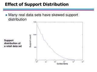
Many real datasets have skewed support distribution, impacting the efficacy of setting minimum support thresholds. This text explores challenges, solutions, and modifications in applying multiple minimum supports for improved association rule mining. From ordering items based on minimum support to mining multi-level and multi-dimensional associations, the text delves into techniques like redundancy filtering and static discretization for quantitative attributes.

E N D
Effect of Support Distribution • Many real data sets have skewed support distribution Support distribution of a retail data set
Effect of Support Distribution • How to set the appropriate minsup threshold? • If minsup is set too high, we could miss itemsets involving interesting rare items (e.g., expensive products) • If minsup is set too low, it is computationally expensive and the number of itemsets is very large • Using a single minimum support threshold may not be effective
Multiple Minimum Support • How to apply multiple minimum supports? • MS(i): minimum support for item i • e.g.: MS(Milk)=5%, MS(Coke) = 3%, MS(Broccoli)=0.1%, MS(Salmon)=0.5% • MS({Milk, Broccoli}) = min (MS(Milk), MS(Broccoli)) = 0.1% • Challenge: Support is no longer anti-monotone • Suppose: Support(Milk, Coke) = 1.5% and Support(Milk, Coke, Broccoli) = 0.5% • {Milk,Coke} is infrequent but {Milk,Coke,Broccoli} is frequent
Multiple Minimum Support (Liu 1999) • Order the items according to their minimum support (in ascending order) • e.g.: MS(Milk)=5%, MS(Coke) = 3%, MS(Broccoli)=0.1%, MS(Salmon)=0.5% • Ordering: Broccoli, Salmon, Coke, Milk • Need to modify Apriori such that: • L1 : set of frequent items • F1 : set of items whose support is MS(1) where MS(1) is mini( MS(i) ) • C2 : candidate itemsets of size 2 is generated from F1instead of L1
Multiple Minimum Support (Liu 1999) • Modifications to Apriori: • In traditional Apriori, • A candidate (k+1)-itemset is generated by merging two frequent itemsets of size k • The candidate is pruned if it contains any infrequent subsets of size k • Pruning step has to be modified: • Prune only if subset contains the first item • e.g.: Candidate={Broccoli, Coke, Milk} (ordered according to minimum support) • {Broccoli, Coke} and {Broccoli, Milk} are frequent but {Coke, Milk} is infrequent • Candidate is not pruned because {Coke,Milk} does not contain the first item, i.e., Broccoli.
Mining Various Kinds of Association Rules • Mining multilevel association • Miming multidimensional association • Mining quantitative association • Mining interesting correlation patterns
uniform support reduced support Level 1 min_sup = 5% Milk [support = 10%] Level 1 min_sup = 5% Level 2 min_sup = 5% 2% Milk [support = 6%] Skim Milk [support = 4%] Level 2 min_sup = 3% Mining Multiple-Level Association Rules • Items often form hierarchies • Flexible support settings • Items at the lower level are expected to have lower support • Exploration of shared multi-level mining (Agrawal & Srikant@VLB’95, Han & Fu@VLDB’95)
Multi-level Association: Redundancy Filtering • Some rules may be redundant due to “ancestor” relationships between items. • Example • milk wheat bread [support = 8%, confidence = 70%] • 2% milk wheat bread [support = 2%, confidence = 72%] • We say the first rule is an ancestor of the second rule. • A rule is redundant if its support is close to the “expected” value, based on the rule’s ancestor.
Mining Multi-Dimensional Association • Single-dimensional rules: buys(X, “milk”) buys(X, “bread”) • Multi-dimensional rules: 2 dimensions or predicates • Inter-dimension assoc. rules (no repeated predicates) age(X,”19-25”) occupation(X,“student”) buys(X, “coke”) • hybrid-dimension assoc. rules (repeated predicates) age(X,”19-25”) buys(X, “popcorn”) buys(X, “coke”) • Categorical Attributes: finite number of possible values, no ordering among values—data cube approach • Quantitative Attributes: numeric, implicit ordering among values—discretization, clustering, and gradient approaches
Mining Quantitative Associations • Techniques can be categorized by how numerical attributes, such as age or salary are treated • Static discretization based on predefined concept hierarchies (data cube methods) • Dynamic discretization based on data distribution (quantitative rules, e.g., Agrawal & Srikant@SIGMOD96) • Clustering: Distance-based association (e.g., Yang & Miller@SIGMOD97) • one dimensional clustering then association • Deviation: (such as Aumann and Lindell@KDD99) Sex = female => Wage: mean=$7/hr (overall mean = $9)
() (age) (income) (buys) (age, income) (age,buys) (income,buys) (age,income,buys) Static Discretization of Quantitative Attributes • Discretized prior to mining using concept hierarchy. • Numeric values are replaced by ranges. • In relational database, finding all frequent k-predicate sets will require k or k+1 table scans. • Data cube is well suited for mining. • The cells of an n-dimensional cuboid correspond to the predicate sets. • Mining from data cubescan be much faster.
Quantitative Association Rules • Proposed by Lent, Swami and Widom ICDE’97 • Numeric attributes are dynamically discretized • Such that the confidence or compactness of the rules mined is maximized • 2-D quantitative association rules: Aquan1 Aquan2 Acat • Cluster adjacent association rules to form general rules using a 2-D grid • Example age(X,”34-35”) income(X,”30-50K”) buys(X,”high resolution TV”)
Mining Other Interesting Patterns • Flexible support constraints (Wang et al. @ VLDB’02) • Some items (e.g., diamond) may occur rarely but are valuable • Customized supmin specification and application • Top-K closed frequent patterns (Han, et al. @ ICDM’02) • Hard to specify supmin, but top-kwith lengthmin is more desirable • Dynamically raise supmin in FP-tree construction and mining, and select most promising path to mine
Pattern Evaluation • Association rule algorithms tend to produce too many rules • many of them are uninteresting or redundant • Redundant if {A,B,C} {D} and {A,B} {D} have same support & confidence • Interestingness measures can be used to prune/rank the derived patterns • In the original formulation of association rules, support & confidence are the only measures used
Interestingness Measures Application of Interestingness Measure
f11: support of X and Yf10: support of X and Yf01: support of X and Yf00: support of X and Y Computing Interestingness Measure • Given a rule X Y, information needed to compute rule interestingness can be obtained from a contingency table Contingency table for X Y Used to define various measures • support, confidence, lift, Gini, J-measure, etc.
Association Rule: Tea Coffee • Confidence= P(Coffee|Tea) = 0.75 • but P(Coffee) = 0.9 • Although confidence is high, rule is misleading • P(Coffee|Tea) = 0.9375 Drawback of Confidence
Statistical Independence • Population of 1000 students • 600 students know how to swim (S) • 700 students know how to bike (B) • 420 students know how to swim and bike (S,B) • P(SB) = 420/1000 = 0.42 • P(S) P(B) = 0.6 0.7 = 0.42 • P(SB) = P(S) P(B) => Statistical independence • P(SB) > P(S) P(B) => Positively correlated • P(SB) < P(S) P(B) => Negatively correlated
Statistical-based Measures • Measures that take into account statistical dependence
Example: Lift/Interest • Association Rule: Tea Coffee • Confidence= P(Coffee|Tea) = 0.75 • but P(Coffee) = 0.9 • Lift = 0.75/0.9= 0.8333 (< 1, therefore is negatively associated)
Drawback of Lift & Interest Statistical independence: If P(X,Y)=P(X)P(Y) => Lift = 1
Interestingness Measure: Correlations (Lift) • play basketball eat cereal [40%, 66.7%] is misleading • The overall % of students eating cereal is 75% > 66.7%. • play basketball not eat cereal [20%, 33.3%] is more accurate, although with lower support and confidence • Measure of dependent/correlated events: lift
Are lift and 2 Good Measures of Correlation? • “Buy walnuts buy milk [1%, 80%]” is misleading • if 85% of customers buy milk • Support and confidence are not good to represent correlations • So many interestingness measures? (Tan, Kumar, Sritastava @KDD’02)
Which Measures Should Be Used? • lift and 2are not good measures for correlations in large transactional DBs • all-conf or coherence could be good measures (Omiecinski@TKDE’03) • Both all-conf and coherence have the downward closure property • Efficient algorithms can be derived for mining (Lee et al. @ICDM’03sub)
There are lots of measures proposed in the literature Some measures are good for certain applications, but not for others What criteria should we use to determine whether a measure is good or bad? What about Apriori-style support based pruning? How does it affect these measures?
Support-based Pruning • Most of the association rule mining algorithms use support measure to prune rules and itemsets • Study effect of support pruning on correlation of itemsets • Generate 10000 random contingency tables • Compute support and pairwise correlation for each table • Apply support-based pruning and examine the tables that are removed
Effect of Support-based Pruning Support-based pruning eliminates mostly negatively correlated itemsets
Effect of Support-based Pruning • Investigate how support-based pruning affects other measures • Steps: • Generate 10000 contingency tables • Rank each table according to the different measures • Compute the pair-wise correlation between the measures
Effect of Support-based Pruning • Without Support Pruning (All Pairs) Scatter Plot between Correlation & Jaccard Measure • Red cells indicate correlation between the pair of measures > 0.85 • 40.14% pairs have correlation > 0.85
Effect of Support-based Pruning • 0.5% support 50% Scatter Plot between Correlation & Jaccard Measure: • 61.45% pairs have correlation > 0.85
Effect of Support-based Pruning • 0.5% support 30% Scatter Plot between Correlation & Jaccard Measure • 76.42% pairs have correlation > 0.85
Subjective Interestingness Measure • Objective measure: • Rank patterns based on statistics computed from data • e.g., 21 measures of association (support, confidence, Laplace, Gini, mutual information, Jaccard, etc). • Subjective measure: • Rank patterns according to user’s interpretation • A pattern is subjectively interesting if it contradicts the expectation of a user (Silberschatz & Tuzhilin) • A pattern is subjectively interesting if it is actionable (Silberschatz & Tuzhilin)
Interestingness via Unexpectedness • Need to model expectation of users (domain knowledge) • Need to combine expectation of users with evidence from data (i.e., extracted patterns) + Pattern expected to be frequent - Pattern expected to be infrequent Pattern found to be frequent Pattern found to be infrequent - + Expected Patterns - + Unexpected Patterns
Interestingness via Unexpectedness • Web Data (Cooley et al 2001) • Domain knowledge in the form of site structure • Given an itemset F = {X1, X2, …, Xk} (Xi : Web pages) • L: number of links connecting the pages • lfactor = L / (k k-1) • cfactor = 1 (if graph is connected), 0 (disconnected graph) • Structure evidence = cfactor lfactor • Usage evidence • Use Dempster-Shafer theory to combine domain knowledge and evidence from data