Download
1 / 36
360 likes | 376 Views
Review of Ozone Performance in WRAP Modeling and Relevance to Future Regional Ozone Planning. Gail Tonnesen, Zion Wang, Mohammad Omary, Chao-Jung Chien University of California, Riverside Zac Adelman University of North Carolina Ralph Morris et al. ENVIRON Corporation Int., Novato, CA.

E N D
Review of Ozone Performance in WRAP Modeling and Relevance to Future Regional Ozone Planning Gail Tonnesen, Zion Wang, Mohammad Omary, Chao-Jung Chien University of California, Riverside Zac Adelman University of North Carolina Ralph Morris et al. ENVIRON Corporation Int., Novato, CA
New 75 ppb eight-hr average NAAQS for ozone will result in increased number of ozone non-attainment areas and the need for new ozone SIPs. New ozone non-attainment areas will be located in western states including rural and remote regions. To what extent can previous WRAP visibility modeling be used to assist in ozone planning? Ozone Planning Needs
Review ozone performance in WRAP regional scale visibility modeling. Assess suitability of 2002 Base Case and 2018 WRAP model results for use as boundary conditions for future high resolution ozone model simulations. Recommend updates and boundary condition values to be used in future ozone modeling studies. White Paper on WRAP Ozone Modeling
Must use photochemical air quality models (CMAQ, CAMx) for ozone SIPs to address several issues: Need to address both 1-hr and 8-hr average. Control strategies might differ in urban versus rural areas. Contributors to ozone include: International transport. Regional transport. local photochemical production: natural & anthropogenic Stratospheric intrusion. Modeling Needs for Ozone
All WRAP CMAQ and CAMx visibility modeling included modeling of ozone: Ozone and other oxidants effect the formation of secondary PM2.5 species sulfate, nitrate and OC. Gas phase NO2 affects visibility directly. Limited evaluation of ozone performance because regional ozone levels have small uncertainty compared to other input data. Previous WRAP Ozone Modeling
2002 Base version B used for the model performance evaluation (MPE): Full year for 36 km model. Selected months for 12km for 2002 Base version A. Planning Cases include: 2002 planning case using typical baseline period emissions (Plan02d). 2018 base case that includes “on the books” emissions reductions (Base18b). Preliminary Reasonable Progress (PRP18a). WRAP Visibility Modeling Cases
Modeling Domain WRAP CMAQ domain: red: 36-km blue: 12-km WRAP 36-km CMAQ/CAMx Domain within MM5 36-km domain
AQS gas phase data includes ozone data at 249 sites in the western US in 2002. Most of the sites in the AQS are for urban influenced sites. Some urban sites also include NO2, CO, HC, SO2. We do not expect the 36 km model to perform well for urban areas because of grid resolution. Limited gas phase data available at rural and remote sites – need more rural gas species monitoring. Review of Previous Ozone MPE
Time-series plots of model and observed data. Spatial plots of model and data. Mean error and bias performance metrics. MPE Results available at: www.cert.ucr.edu/aqm/308/cmaq.shtml #base02aV4512kvs36k #base02bvsbase02a36k Model Performance Approach
Tabulated Fractional Bias and Error(using 60 ppb filter for observed data)
Tabulated Fractional Bias and Error(using 60 ppb filter for observed data)
Limited monitoring data available for rural and remote sites. 12km model was not superior to 36km model. CMAQ performed well for ozone for remote sites (although data for MPE was very limited). Tabulated metrics shown above are not appropriate for rural ozone MPE because of 60 ppb filter and the predominance of urban sites. Summary for Ozone MPE
Need to identify rural and upwind urban sites in AQS database for more complete MPE, and need to add new monitoring sites. Explore use of satellite data for ozone, NO2 and other gas species. Need aloft measurements and ocean aloft measurements to better characterize transport. Develop new metrics for MPE that do not employ the 60 ppb ozone filter. Future Needs for Ozone MPE
Compare Base 2018 Base Case and 2018 Preliminary Reasonable Progress Case to the 2002 Planning Case for benefits on ozone reduction. Results available on RMC webpage: www.cert.ucr.edu/aqm/308/cmaq.shtml #base18bvsplan02b #prp18avsplan02d Results include daily average, monthly average and annual average spatial difference plots. Projected Ozone for 2018
Reductions in monthly average ozone of 1 to 10 ppb during summer in 2018 Base Case. Slightly larger reductions in 2018 PRP case. PRP18a case predicts exceedence of the 8-hr average ozone standard in much of the southwestern US, mostly in spring. Likely that there is large contribution from tranported ozone. Need to re-evaluate GEOSCHEM ozone BC. Summary of 2018 Ozone Predictions
Emissions data – largest uncertainty, ranges from 30% to a factor of 3 depending on source category. WRAP made significant improvements in emissions, largest uncertainties remain in biogenic VOC, and NH3. Meteorology, vertical mixing and PBL height – can have large effect on model performance, especially for urban areas. Need to compare MM5 and WRF. Boundary conditions – we have pretty good BC estimates from GEOSCHEM. Larger uncertainty in ozone at model top and in the future BC and transport. Uncertainty related to future climate – probable increases in biogenic VOC and in reactivity. Uncertainties in Input Data
Photochemical mechanisms – gas phase ozone chemistry is best for rural low NOx conditions. Mechanisms underestimate reactivity for urban high NOx conditions. Heterogeneous and aqueous chemistry – potentially largest uncertainty affecting regional ozone formation. Large uncertainty in NOx budget and fate of NOx (N2O5 hydrolysis, renoxification, HOx radical budgets). Grid resolution effects – artificial dispersion might over estimate ozone formation in areas with large emissions. Also makes MPE more difficult. Nested grids in CAMx can better handle urban ozone budgets. Uncertainties in Model Science
Existing planning cases and 2002 base case are useful for evaluating ozone in rural & remote areas. Sensitivity studies can be performed to estimate effects of boundary conditions and sensitivity to emissions controls, either across the board emissions reductions or by source category. Data can be extracted from 2002 base case to create BC for new, high resolution 4-km ozone modeling. Applications of WRAP data
Ozone can be reduced by controlling both VOC and NOx. Urban ozone in the west is more sensitive to VOC control, while NOx controls can have both benefits and transient dis-benefits for urban ozone. (There is no NOx dis-benefit for urban ozone if NOx reductions are sufficiently large.) Rural ozone is more sensitive to NOx controls. Ozone sensitivity to VOC and NOx reductions can be estimated directly using ambient indicator ratios (although data is limited) and using model sensitivity simulations. Ozone Sensitivity to VOC and NOx
Ozone produced per molecule of NOx emissions varies considerably – less efficient ozone production at low VOC/NOx ratios and at higher VOC and NOx concentrations because NOx is more rapidly converted to inert HNO3: Power plant plumes: 1-3 molecules O3 per NOx Urban conditions: 4-10 molecules O3 per NOx Rural conditions: 10-100 molecules O3 per NOx Much greater benefit of controlling mobile and areas sources of NOx in rural areas for an equivalent mass reduction. Ozone Production Efficiency per NOx
New emissions data should be included in future CMAQ or CAMx runs: MEGAN biogenic model; new oil & gas inventory; lightning NOx emissions. Should use updated model versions and updated chemistry, new CB-05 or new SAPRC07, if available. Updated global simulations for present and future BC. Need to save 3-d concentration files in all future runs. Long-term needs: More ambient monitoring of gas species. Advances in science of NOx budget and fate. Recommended Model Updates