Download
1 / 32
320 likes | 519 Views
Types of measurements in superconductivity. Adrian Crisan School of Metallurgy and Materials, University of Birmingham, UK a nd National Institute of Materials Physics, Bucharest, Romania. CONTENTS. I. Transport measurements II. DC magnetization III. AC susceptibility.

E N D
Types of measurements in superconductivity Adrian Crisan School of Metallurgy and Materials, University of Birmingham, UK and National Institute of Materials Physics, Bucharest, Romania
CONTENTS • I. Transport measurements • II. DC magnetization • III. AC susceptibility
I. Transport measurements • Contacts: rather easy for wires/tapes (soldering with low temperature soldering alloys based on Indium), quite easy for bulk and melt-textured (Silver paste), and quite difficult for films • Need to use photolitography (photoresist S1818,UV400 Exposure Optics, Karl Suss MJB3 Mask Aligner, Microsposit MF-319 developer) and etching (Diluted Nitric acid 0.1% ) to produce micron-sized bridges
An overview of 4 bridges after etching Karl Suss MJB3 Mask Aligner system
Scheme of rotation measurement of YBCO bridge Quantum Design SQUID MPMS Q.D. PPMS looks rather similar
Resistivity vs. temperature: Tc(H), magnetoresistance Resistivity transition of 1μm BZO-doped YBCO film in magnetic fields of 0, 0.5, 1, 2, 3, 4, 5 and 6 T with H//c Resistivity transition of 1μm BZO-doped YBCO film in magnetic fields of 0, 0.5, 1, 2, 3, 4, 5 and 6 T with H//ab
Phase diagram of High-Tc superconductors The vortex lattice undergoes a first-order melting transition transforming the vortex solid into a vortex liquid [Fisher et al, PRB 43,130, 1991]. At low magnetic fields (approx 1 Oe in BSCCO [A.C. et al, SuST 24, 115001, 2011), there is a reentrance of the melting line [Blatter et al, PRB 54, 72, 1996]. The flux lines in the vortex -liquid are entangled resulting in an ohmic longitudinal response, hence the vortex liquid and normal metallic phases are separated by a crossover at Hc2. • Low enough currents • VL- linear dissipation: E ≈ J • VS (VGlass)- strongly nonlinear dissipation: E ≈ exp[-(JT/J)m]
Vortex melting from transport measurements I-V curves of [(BaCuO2)2/(CaCuO2)2]×35 artificial superlattices in three magnetic fields. The dashed lines represent power-law fits at the chosen melting temperatures: a) B=0.55 kG, T between 57 and 79.8 K, Tm=72.8 K; b) B=4.4 kG, T between 55.85 and 78.1 K, Tm=70.9 K; and c) B=10.8 kG, T between 49.75 and 75.4 K, Tm=68.1 K. YBCO single-grain [A. C. et al, Physica C 313, 70, 1999] [A. C. et al, Physica C 355, 231, 2001]
Above Tm(B), the I–V curves crossover from an Ohmic behaviour at low currents to a power-law relation at high currents and every I–V curve displays an upward curvature. Below Tm(B), the I–V curves show an exponential relation at low currents and a power-law behaviour at high currents, with a downward curvature, suggesting that the system approaches to a truly superconducting phase VG for J exponentially small. At Tm(B), where the crossover between downward and upward curvatures occurs, the whole I–V curve displays a power-law relation, which takes the form: V (I, T=Tm) ≈ I(z+1)/(d-1), where z is the critical dynamical exponent of VG, and d dimensionality of the system (3 in this case). Above Tm(B) and for low currents, the Ohmic region in the I–V curves, the linear resistance Rl(T) can be scaled as: Rl ≈ (T/Tm-1)n(z+2-d), where n is the static critical exponent.
Fisher, Fisher, Huse scaling (PRB 43, 130, 1991)
Angle dependence of critical current (15Ag/1mm BZO-doped YBCO)x2
Dependence of Ic on the field orientation for (Ag/(YBCO+BZO))x3, showing a small anisotropy for intermediate fields.
II. DC magnetization Jc=Ct.DM Depends strongly on sample geometry thin films; m=DM/2; d-thickness; a,b-rectangle dimension:
Field dependence of the critical current at 77 K for some quasi-multilayers grown in Birmingham in comparison with some results of other EU groups (green and black symbols)
Bulk pinning force • Fp=BxJc 2.33h1/2(1-h)2+1.5h(1-h)2+0.63h(1-h) Surface normal (65%), point normal (22%), volume Dk (13%) 3.15h1/2(1-h)2+0.57h(1-h)2+0.19h3/2(1-h) Surface normal (90%), point normal (8%), surface Dk (2%)
III. AC susceptibility measurements • fundamental and 3rdharmonic • Quantum Design PPMS • (T) at various HDC, hac ( 15 Oe), f ( 10 kHz): Tc(H) • ”(hac), 3(hac) at various fixed T and HDC and varying f: Jc(T,HDC, f), Ueff(T,HDC) Tm is the on-set of third harmonic susceptibility 3(T) [A. C. et al., 2003 Appl. Phys. Lett. 83 506]
Critical current density as function of temperature, field, and frequency, using AC susceptibility measurements • JC = h*/da (in A/cm2) • h* - position of maximum (in Oe) • d – film thickness (in cm) • - coefficient slightly dependent on geometry (approx. 0.9) • E.H. Brandt, Physical Review B • 49/13 (1994) 9024.
Anderson-Kim Collective pinning Zeldov
EXPERIMENTAL: A.C. et al, SuST 22, 045014, 2009
Vortex melting line from ac susceptibility ” is a measure of total dissipation: -linear: Thermal Activated Flux Flow (TAFF) and Flux Flow (FF) -nonlinear:Flux Creep 3 is a measure on nonlinear dissipation (flux-creep) only [P. Fabricatore et al, PRB 50, 3189, 1994]
-two-fluid: ab(T)= ab(0)[1–(T/Tc)4]-1/2 -3D XY : ab(T)= ab(0)[1–T/Tc]-1/3 -mean-field: ab(T)= ab(0)[1–T/Tc]-1/2 C 1/42 , cL = 0.15, =90
Examples 3D XY Two-fluid gYBCO = 5.4 gTl:1223=12.6 [A. C. et al., 2003 Appl. Phys. Lett. 83 506] [A. C. et al., 2007 PRB 76 21258]
n=9 9 HgBa2O2 13 14 9 8 c 6 9 a 8 10 Z O(1)2- OP (SC) Nh IP (AF) (n-2) -(z) OP (SC) O(2)2- HgBa2Can-1CunOy (with n ≥ 6 ) [A. C. et al., 2008 PRB 77 144518]
Two-fluid (1245 and 1234) Magnetically-coupled pancake vortex molecules composed of two pancakes separated by the thin CRL, strongly coupled by Josephson coupling
Ba2Ca3Cu4O8(O1−yFy)2 [ F(2y)-0234] • Ba2Can-1CunO2n+2 (n=3-5), F=0, samples are optimally doped with Tc larger than 105 K, but they are very unstable • The system becomes stable after substitution of F at the apical O site; underdoped states • F(2.0)-0234 is not a Mott insulator, but a SC with Tc=58 K • Thin CRL (0.74 nm) as compared with other multilayered cuprates • Allow the investigation of underdoped region by varying the F doping • 2y = 1.3, 1.6, 2.0 (105, 86, 58 K) [D. D. Shivagan,.., A.C., et al., SuST 24, 095002]
Penetration depth: 3D XY critical fluctuations model • F(1.3)-0234 near-optimally-doped, enough carriers in both OP and IPs, 3D SC, strong Josephson coupling
Penetration depth: mean-field model • F(1.6)-0234 under-doped; out of the region of critical fluctuations; rearrangement of Fermi surfaces through hybridization between OP and IP bands; OP Fermi surface has a 2D character, IP Fermi surface has a 3D character
Penetration depth: two-fluid model • F(2.0)-0234 heavily under-doped; formal Cu valence is 2+, should be half-filled Mott insulator; evidence of self-doped thick IPs block, as compared with thin IP block of F(2.0)-0212 that shows 3D-2D cross-over • Absence of 3D-2D cross-over is a manifestation of cooperative coupling in CRL and IPs