Download
1 / 35
350 likes | 565 Views
Analysis and numerical modeling of Galveston shoreline change – implications for erosion control. Dr. Tom Ravens and Khairil Sitanggang Texas A&M University at Galveston Supported by Texas Sea Grant, Texas GLO Galveston County, Texas A&M, Corps of Engineers. Study objectives.

E N D
Analysis and numerical modeling of Galveston shoreline change – implications for erosion control Dr. Tom Ravens and Khairil Sitanggang Texas A&M University at Galveston Supported by Texas Sea Grant, Texas GLO Galveston County, Texas A&M, Corps of Engineers
Study objectives • To determine (quantify) the processes responsible for beach change • Longshore sediment transport • Cross-shore sediment transport • To use that knowledge to design effective and realistic erosion control measures
Longshore sediment transport Qls = C Hb5/2 sin 2ab
Erosional Hot Spot due to blocked longshore transport Longshore transport Groin field South Jetty Erosional hotspot Galveston Island State Park
Instrument sled for transport measurement What is C in {Qls = C Hb5/2 sin 2ab}?
Offshore transport due to storms erosion deposition Is offshore transport permanent?
Limitations to direct calculation of beach change from processes • Available WIS wave data (1990-2001) leads to sediment transport predictions in direction opposite of observed direction. • No easy way to calculate cross-shore transport
Alternative (indirect) approach • Analyze shoreline data (1956, 65, 90, and 2001) with a sediment budget and infer longshore and cross-shore transport indirectly • Identify period (1990-2001) which was dominated by longshore transport • Use longshore data (from 1990-2001) to screen and select wave data which can then be used for detailed design of shoreline protection measures
Sediment budget to estimate long- and cross-shore transport DV DV = Qin - Qout
Estimating Volume Change From Shoreline Change Rate de Hb Dc Equilibrium profiles DV = (Hb+Dc) de [m3/m]
East End Sediment Budget Compartment 1 Compartment 2 3 km 2.5 km Q = 0 Q = 6000m3/yr Q = 41,000 m3/yr DV = 41,000 m3/yr DV = -35,000 m3/yr South jetty
Apparent westward longshore transport 180,000 m3/yr average
Year Selected hurricanes and tropical storms (1956-2001) Maximum storm surge at Galveston Gulf shoreline Number of hours with storm surge above 1.5 m 1957 Audrey ??? ??? 1961 Carla 2.75 55 1980 Allen 1.1 0 1983 Alicia 2.4 7 1996 Josephine 1.0 0 1998 Frances 1.4 0 2001 Allison 0.9 0 Storms 1956-2001
Wave and potential sediment transport calculations on west end *Station 1079
Predicted and measured 2001 shoreline(based on 1977, 1979,1982,1989, 1991 waves) Distance Offshore (m) 1990 2001 measured 2001 calculated
Predicted 2011 shoreline as a function of beach nourishment 2001 2011 100,000 m3/yr 2011 no nourishment
Offshore breakwater shifts erosion hotspot down drift breakwater 2001 2011
Designing erosion control measures for hurricanes • Approach: use wave data to calculate longshore transport for 1956-65, 1965-90 • Use measured volume change for these periods • Infer offshore transport rates based on sediment budget concept • Find offshore transport rates of about 500,000 m3/yr • Expect to spend about $3,000,000 to $5,000,000 per year (if 1956-1990 trend returns)
Determining offshore sediment transport and sand needs under storm conditions Qoffshore = 500,000 m3/y DV Qoffshore = = Qin – Qout - DV
Who blocks the sand? South jetty Gulf of Mexico State Park Galveston
Conclusions • Sediment budget effective tool for estimating longshore transport and cross-shore transport • Modeling (neglecting hurricanes) indicates about 100,000 m3/yr needed for hotspot • Much more sand (~500,000 m3/yr) would be needed for west end if hurricanes return • Majority of erosion on west end is due to storm-induced cross-shore transport • Groin field suffers relatively little storm-induced erosion • Tropical storms do not cause permanent loss of sand
DV = 6,000 m3/yr (64,000) 6,000 m3/yr (64,000) DV = -69,000 m3/yr (-18,000) (67,000) 63,000 m3/yr DV = -309,000 m3/yr (20,000) (-155,000) DV = -255,000 m3/yr 371,000m3/yr (220,000) (175,000) 778,000 m3/yr (-45,000)
Interpretation of “Calculated” Longshore Transport • Very high longshore transport calculated for 1956-65 and for 1965-90 probably due to neglecting cross-shore transport associated with Hurricanes Carla and Alicia • Cross-shore transport probably from the beach/nearshore to the offshore • Little evidence of over wash during Alicia • Dellapenna data indicates significant sand deposition into the mud beyond the depth of closure. • Assume 4 cm/yr deposition, 20% sand, 50 km x 5 km area, • Calculate: 2 million m3/yr cross-shore transport
Conclusions • Calculating changes in sediment volume based on shoreline change appears to underestimate volume change somewhat. • Calculations of longshore transport based on offshore wave conditions appears uncertain. • Sediment budget/flows are a function of time especially at the west end of the island
Future Work • Account for other flows besides wave-derived longshore transport in the surf zone. • Account for the build up of sediment at big reef (which suggests transport across the south jetty) and possible cross-shore transport at the East Beach. • We need to better understand the dynamics of San Luis Pass and the role it plays on the sediment budget.
DV = 6,000 m3/yr (64,000) 6,000 m3/yr (64,000) DV = -69,000 m3/yr (-18,000) (67,000) 63,000 m3/yr DV = -309,000 m3/yr (20,000) (-155,000) DV = -255,000 m3/yr 371,000m3/yr (220,000) (175,000) 778,000 m3/yr (-45,000)
Analysis of shoreline data from Galveston Island • Sediment budget based on shoreline data (1956, 1965, 1990, 2001) • Identify stormy periods (with cross-shore transport) and calm periods • Quantification of cross-shore and longshore transport during different periods of time • GENESIS modeling during 1990-2001 • Design of beach nourishment 2001-2011.
Estimating Volume Change From Shoreline Change Rate de Hb Dc Equilibrium profiles DV = (Hb+Dc) de [m3/m]