
Spatial Analysis Using Grids
E N D
Presentation Transcript
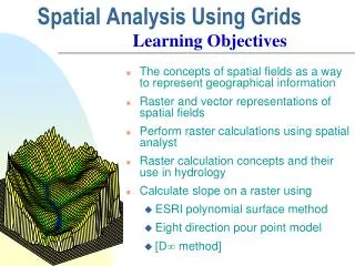
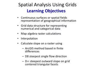
Spatial Analysis Using Grids Learning Objectives By the end of this class you should be able to: • describe some ways continuous surfaces or spatial fields are represented in GIS • list and describe the data elements that comprise a grid data structure • describe how integer, categorical and real valued data fields are represented using grids • use map algebra to perform raster calculations on grids and explain the scale issues involved in raster calculations where grids may not have the same cell size • define interpolation and describe aspects to be considered in interpolating a spatial field • use interpolation to determine watershed average precipitation (Ex 3) • calculate the slope of a topographic surface represented by a grid using: • ArcGIS method based on finite differences, • D8 model in direction of steepest single flow direction, • D model in direction of steepest outward slope on grid centered triangular facets.
Readings - Theory • ArcMap help: What is raster data? http://desktop.arcgis.com/en/arcmap/latest/manage-data/raster-and-images/what-is-raster-data.htm • ArcMap help: Fundamentals of raster data from Cell size of raster data to Raster dataset attribute tables http://desktop.arcgis.com/en/arcmap/latest/manage-data/raster-and-images/cell-size-of-raster-data.htm
Readings – ArcGIS Pro Tools • ArcGIS Pro An overview of the Spatial Analyst Toolbox https://pro.arcgis.com/en/pro-app/tool-reference/spatial-analyst/an-overview-of-the-spatial-analyst-toolbox.htm. Read this to get a general sense of the tools available. Tools we will use now or later include, from the Surface toolset: Slope, Aspect, Contour; from the Zonal toolset: Zonal Statistics; from Map Algebra: Raster Calculator; from Interpolation: Spline and Kriging; and many tools in the Hydrology toolset.
Readings – Slope and Aspect • How Slope Works https://pro.arcgis.com/en/pro-app/tool-reference/spatial-analyst/how-slope-works.htm • How Aspect Workshttps://pro.arcgis.com/en/pro-app/tool-reference/spatial-analyst/how-aspect-works.htm
Slope Handout http://hydrology.usu.edu/dtarb/giswr/2017/Slope.pdf Determine the length, slope and azimuth of the line AB.
(x1,y1) y f(x,y) x Two fundamental ways of representing geography are discrete objects and fields. The discrete object view represents the real world as objects with well defined boundaries in empty space. Features (Shapefiles) Points Lines Polygons The field viewrepresents the real world as a finite number of variables, each one defined at each possible position. Rasters Continuous surface
Numerical representation of a spatial surface (field) Grid or Raster TIN Contour and flowline
Raster and Vector Data Raster data are described by a cell grid, one value per cell Vector Raster Point Line Zone of cells Polygon
Polygon as Zone of Grid Cells From: http://resources.arcgis.com/en/help/main/10.2/index.html#/How_features_are_represented_in_a_raster/009t00000006000000/
Raster and Vector are two methods of representing geographic data in GIS • Both represent different ways toencode andgeneralizegeographic phenomena • Both can be used to code both fields and discrete objects • In practice a strong association between raster and fieldsand vector and discrete objects
A grid defines geographic space as a mesh of identically-sized square cells. Each cell holds a numeric value that measures a geographic attribute (like elevation) for that unit of space.
The grid data structure Number of Columns • Grid size is defined by extent, spacing and no data value information • Number of rows, number of column • Cell sizes (X and Y) • Top, left , bottom and right coordinates • Grid values • Real (floating decimal point) • Integer (may have associated attribute table) Number of rows Cell size (X,Y) NODATA cell
Floating Point Grids Continuous data surfaces using floating point or decimal numbers
Value attribute table for categorical (integer) grid data Attributes of grid zones
Raster Sampling from Michael F. Goodchild. (1997) Rasters, NCGIA Core Curriculum in GIScience, http://www.ncgia.ucsb.edu/giscc/units/u055/u055.html, posted October 23, 1997
Cell size of raster data From http://help.arcgis.com/en/arcgisdesktop/10.0/help/index.html#/Cell_size_of_raster_data/009t00000004000000/
Raster Generalization Largest share rule Central point rule
Map Algebra/Raster Calculation Example 5 6 Precipitation - Losses (Evaporation, Infiltration) = Runoff 7 6 Cell by cell evaluation of mathematical functions - 3 3 2 4 = 2 3 5 2
Cell based discharge mapping by accumulation of generated runoff Radar Precipitation grid Soil and land use grid Runoff grid from raster calculator operations implementing runoff generation formula’s Accumulation of runoff within watersheds
Raster calculation – some subtleties Resampling or interpolation (and reprojection) of inputs to target extent, cell size, and projection within region defined by analysis mask + = Analysis mask Analysis cell size Analysis extent
2.2 3 4 1.8 2.5 3.5 1.5 2 2.7 Runoff Generation Raster Calculation Example Precipitation, P cm/hr Infiltration Rate, f cm/hr 150 m 100 m 100 m 150 m 4 6 3.1 4 Runoff R = P-f
Lets Experiment with this in ArcGIS precip.asc ncols 2 nrows 2 xllcorner 0 yllcorner 0 cellsize 150 NODATA_value -9999 4 6 3.1 4 infiltration.asc ncols 3 nrows 3 xllcorner 0 yllcorner 0 cellsize 100 NODATA_value -9999 2.2 3 4 1.8 2.5 3.5 1.5 2 2.7
Runoff calculation using Raster Calculator “precip.asc” - “infiltration.asc”
The Result • Outputs are on 150 m grid. • How were values obtained ? 1.8 2 1.6 1.3
2.2 4 3 1.8 2.5 3.5 150 m 6 4 1.5 2 2.7 3.1 4 Nearest Neighbor Resampling with Cellsize Maximum of Inputs 100 m 4 - 2.2 = 1.8 6 - 4 = 2 1.8 2 3.1 – 1.5 = 1.6 4 – 2.7= 1.3 1.6 1.3
Inferences • ArcGIS has used nearest neighbors to align cells • ArcGIS has done raster computation at the scale of the coarsest input • Is this what we want? • How to control scale? • What is meant by scale in this context?
The scale triplet a) Extent b) Spacing c) Support From: Blöschl, G., (1996), Scale and Scaling in Hydrology, Habilitationsschrift, Weiner Mitteilungen Wasser Abwasser Gewasser, Wien, 346 p.
Scale and the interpretation of data From: Blöschl, G., (1996), Scale and Scaling in Hydrology, Habilitationsschrift, Weiner Mitteilungen Wasser Abwasser Gewasser, Wien, 346 p.
Resample to get consistent cell size Spacing & Support Method 4 5 6 6 4 5 3.55 4.275 4 3.1 3.1 3.55 4
Calculation with consistent 100 m cell size grid “precip100” - “infiltration” • Outputs are on 100 m grid as desired. • How were values obtained ? 1.8 2 2 1.75 1.775 1.5 1.6 1.55 1.3
100 m 2.2 4 3 2.5 3.5 1.8 1.5 2 2.7 100 m cell size raster calculation 4 – 2.2 = 1.8 5 – 3 = 2 6 – 4 = 2 3.55 – 1.8 = 1.75 4.275 – 2.5 = 1.775 5 – 3.5 = 1.5 1.8 2 2 3.1 – 1.5 = 1.6 5 6 4 100 m 3.55 – 2 = 1.55 5 1.75 1.775 1.5 4 – 2.7 = 1.3 3.55 4.275 3.1 3.55 4 1.6 1.55 1.3
Interpolation Estimate values between known values. A set of spatial analyst functions that predict values for a surface from a limited number of sample points creating a continuous raster. • Nearest neighbor • Inverse distance weight • Bilinear interpolation • Kriging (best linear unbiased estimator) • Spline
Interpolation Comparison Grayson, R. and G. Blöschl, ed. (2000)
Further Reading Grayson, R. and G. Blöschl, ed. (2000), Spatial Patterns in Catchment Hydrology: Observations and Modelling, Cambridge University Press, Cambridge, 432 p. Chapter 2. Spatial Observations and Interpolation Full text online at: http://www.hydro.tuwien.ac.at/forschung/publikationen/engl-publikationen/spatial-patterns-in-catchment-hydrology.html
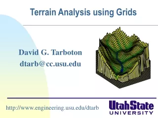
Analysis of topographic surfaces represented by a Digital Elevation Model (DEM) 3-D detail of the Tongue river at the WY/Mont border from LIDAR. Roberto Gutierrez University of Texas at Austin
Topographic Slope • Defined or represented by one of the following • Surface derivative z. Given z(x,y) evaluate (dz/dx, dz/dy) • Vector with x and y components (Sx, Sy) • Vector with magnitude (slope) and direction (aspect) (S, ) See http://hydrology.usu.edu/dtarb/giswr/2018/Slope.pdf
Slope and Aspect = aspect clockwise from North https://pro.arcgis.com/en/pro-app/tool-reference/spatial-analyst/how-slope-works.htm
a b c d e f g h i ArcGIS “Slope” tool y Similarly Slope magnitude = x c b f a e i d h g x y
ArcGIS Aspect – the steepest downslope direction Use atan2 to resolve ambiguity in atan direction https://pro.arcgis.com/en/pro-app/tool-reference/spatial-analyst/how-aspect-works.htm
Example a b c 30 d e f 145.2o 80 74 63 69 67 56 g h i 60 52 48
80 80 74 74 63 63 69 69 67 67 56 56 60 60 52 52 48 48 Hydrologic Slope (Flow Direction Tool) - Direction of Steepest Descent 30 30 Slope:
32 64 128 16 1 8 4 2 Eight Direction Pour Point Model ESRI Direction encoding
? Limitation due to 8 grid directions.
The D Algorithm Tarboton, D. G., (1997), "A New Method for the Determination of Flow Directions and Contributing Areas in Grid Digital Elevation Models," Water Resources Research, 33(2): 309-319.) (http://www.engineering.usu.edu/cee/faculty/dtarb/dinf.pdf)
The D Algorithm z0 Elevations at each vertex zi z2 z1 If 1 does not fit within the triangle the angle is chosen along the steepest edge or diagonal resulting in a slope and direction equivalent to D8
D∞ Example 30 80 74 63 69 67 56 60 52 48 284.9o 14.9o eo e8 e7 From ArcGIS Pro Help: