
Thread-Level Parallelism in Multicore Processors
E N D
Presentation Transcript
Thread-Level Parallelism Instructor: Adam C. Champion, Ph.D. CSE 2431: Introduction to Operating Systems Reading: Section 12.6, [CSAPP]
Contents • Parallel Computing Hardware • Multicore: Multiple separate processors on single chip • Hyperthreading: Replicated instruction execution hardware in each processor • Maintaining cache consistency • Thread Level Parallelism • Splitting program into independent tasks • Example: Parallel summation • Some performance artifacts • Divide-and-conquer parallelism • Example: Parallel quicksort
Multicore Processor Core 0 Core n – 1 • Intel Nehalem Processor • E.g., Shark machines (Xeon E5520 CPU, 2.27 GHz, 8 cores, [2 threads each]) • Multiple processors operating with coherent view of memory • Use /proc/cpuinfo to see CPU info (Linux) Regs Regs L1 d-cache L1 i-cache L1 d-cache L1 i-cache … L2 unified cache L2 unified cache L3 unified cache (shared by all cores) Main memory
Memory Consistency int a = 1; int b = 100; • What are the possible values printed? • Depends on memory consistency model • Abstract model of how hardware handles concurrent accesses • Sequential consistency • Overall effect consistent with each individual thread • Otherwise, arbitrary interleaving Thread consistency constraints Wa Rb Thread1: Wa: a = 2; Rb: print(b); Thread2: Wb: b = 200; Ra: print(a); Wb Ra
Sequential Consistency Example Thread consistency constraints int a = 1; int b = 100; Wa Rb • Impossible outputs • 100, 1and 1, 100 • Would require reaching both Ra and Rb before Wa and Wb Wb Ra Thread1: Wa: a = 2; Rb: print(b); Thread2: Wb: b = 200; Ra: print(a); 100, 2 Rb Wb Ra Wa Rb Ra 200, 2 Wb 2, 200 Ra Rb 1, 200 Ra Wa Rb 2, 200 Wb Ra Rb Wa Rb Ra 200, 2
Non-Coherent Cache Scenario int a = 1; int b = 100; • Write-back caches, without coordination between them Thread1: Wa: a = 2; Rb: print(b); Thread2: Wb: b = 200; Ra: print(a); a:1 b:100 print 1 print 100 Thread1 Cache Thread2 Cache a: 2 b:200 Main Memory a:1 b:100
Snoopy Caches (1) int a = 1; int b = 100; • Tag each cache block with state Invalid Cannot use value Shared Readable copy Exclusive Writeable copy Thread1: Wa: a = 2; Rb: print(b); Thread2: Wb: b = 200; Ra: print(a); Thread1 Cache Thread2 Cache E a: 2 E b:200 Main Memory a:1 b:100
Snoopy Caches (2) int a = 1; int b = 100; • Tag each cache block with state Invalid Cannot use value Shared Readable copy Exclusive Writeable copy Thread1: Wa: a = 2; Rb: print(b); Thread2: Wb: b = 200; Ra: print(a); Thread1 Cache Thread2 Cache E S a: 2 a: 2 S a:2 print 2 E b:200 S b:200 S b:200 print 200 Main Memory • When cache sees request for one of its E-tagged blocks • Supply value from cache • Set tag to S a:1 b:100
Out-of-Order Processor Structure Instruction Control Instruction Cache • Instruction control dynamically converts program into stream of operations • Operations mapped onto functional units to execute in parallel Functional Units Instruction Decoder Integer Arith Integer Arith FP Arith Load / Store Registers Op. Queue PC Data Cache
Hyperthreading Instruction Control Instruction Cache • Replicate enough instruction control to process K instruction streams • K copies of all registers • Share functional units Functional Units Instruction Decoder Reg A Op. Queue A Integer Arith Integer Arith FP Arith Load / Store Reg B Op. Queue B PC A PC B Data Cache
Summary: Creating Parallel Machines • Multicore • Separate instruction logic and functional units • Some shared, some private caches • Must implement cache coherency • Hyperthreading • Also called “simultaneous multithreading” • Separate program state • Shared functional units & caches • No special control needed for coherency • Combining • Shark machines: 8 cores, each with 2-way hyperthreading • Theoretical speedup of 16× (Never achieved in benchmarks)
Summation Example • Sum numbers 0, …, N – 1 • Should add up to (N – 1) * N / 2 • Partition into K ranges • N/K values each • Each thread sums one range of numbers • Assume that N is a multiple of K (for simplicity)
Example 1: Parallel Summation • Sum numbers 0, …, n – 1 • Should add up to ((n–1)*n)/2 • Partition values 1, …, n – 1into t ranges • n/t values in each range • Each of t threads processes 1 range • For simplicity, assume n is a multiple of t • Let’s consider different ways that multiple threads might work on their assigned ranges in parallel
First attempt: psum-mutex (1) • Simplest approach: Threads sum into a global variable protected by a semaphore mutex. void *sum_mutex(void *vargp); /* Thread routine */ /* Global shared variables */ longgsum = 0; /* Global sum */ longnelems_per_thread; /* Number of elements to sum */ sem_tmutex; /* Mutex to protect global sum */ intmain(intargc, char **argv) { longi, nelems, log_nelems, nthreads, myid[MAXTHREADS]; pthread_ttid[MAXTHREADS]; /* Get input arguments */ nthreads = atoi(argv[1]); log_nelems = atoi(argv[2]); nelems = (1L << log_nelems); nelems_per_thread = nelems / nthreads; sem_init(&mutex, 0, 1); psum-mutex.c
psum-mutex (2) • Simplest approach: Threads sum into a global variable protected by a semaphore mutex. /* Create peer threads and wait for them to finish */ for (i = 0; i < nthreads; i++) { myid[i] = i; Pthread_create(&tid[i], NULL, sum_mutex, &myid[i]); } for (i = 0; i < nthreads; i++) Pthread_join(tid[i], NULL); /* Check final answer */ if (gsum != (nelems * (nelems-1))/2) printf("Error: result=%ld\n", gsum); return 0; } psum-mutex.c
psum-mutex Thread Routine • Simplest approach: Threads sum into a global variable protected by a semaphore mutex. /* Thread routine for psum-mutex.c */ void *sum_mutex(void *vargp) { longmyid = *((long *)vargp); /* Extract thread ID */ longstart = myid * nelems_per_thread; /* Start element index */ longend = start + nelems_per_thread; /* End element index */ longi; for (i = start; i < end; i++) { P(&mutex); gsum += i; V(&mutex); } returnNULL; } psum-mutex.c
psum-mutexPerformance • Shark machine with 8 cores, n = 231 • Nasty surprise: • Single thread is very slow • Gets slower as we use more cores
Next Attempt: psum-array • Peer thread i sums into global array element psum[i] • Main waits for threads to finish, then sums elements of psum • Eliminates need for mutex synchronization /* Thread routine for psum-array.c */ void *sum_array(void *vargp) { longmyid = *((long *)vargp); /* Extract thread ID */ longstart = myid * nelems_per_thread; /* Start element index */ longend = start + nelems_per_thread; /* End element index */ longi; for (i = start; i < end; i++) { psum[myid] += i; } returnNULL; } psum-array.c
psum-array Performance • Orders of magnitude faster than psum-mutex
Next Attempt: psum-local • Reduce memory references by having peer thread i sum into a local variable (register) /* Thread routine for psum-local.c */ void *sum_local(void *vargp) { longmyid = *((long *)vargp); /* Extract thread ID */ longstart = myid * nelems_per_thread; /* Start element index */ longend = start + nelems_per_thread; /* End element index */ longi, sum = 0; for (i = start; i < end; i++) { sum += i; } psum[myid] = sum; returnNULL; } psum-local.c
psum-local Performance • Significantly faster than psum-array
Characterizing Parallel Program Performance • p processor cores, Tk is the running time using k cores • Speedup:Sp = T1 / Tp • Spis relative speedup if T1 is running time of parallel version of the code running on 1 core. • Sp is absolute speedup if T1 is running time of sequential version of code running on 1 core. • Absolute speedup is a much truer measure of the benefits of parallelism. • Efficiency:Ep = Sp/p = T1/(pTp) • Reported as a percentage in the range (0, 100]. • Measures the overhead due to parallelization
Performance of psum-local • Efficiencies OK, not great • Our example is easily parallelizable • Real codes are often much harder to parallelize (e.g., parallel quicksort later in this lecture)
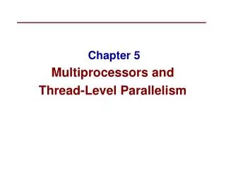
Amdahl’s Law Gene Amdahl (Nov. 16, 1922 – Nov. 10, 2015) • Captures the difficulty of using parallelism to speed things up. • Overall problem • T: Total sequential time required • p: Fraction of total that can be sped up (0 p 1) • k: Speedup factor • Resulting Performance • Tk = pT/k + (1 – p)T • Portion which can be sped up runs k times faster • Portion which cannot be sped up stays the same • Least possible running time: • k = • T = (1 – p)T
Amdahl’s Law Example • Overall problem • T = 10 Total time required • p = 0.9 Fraction of total which can be sped up • k = 9 Speedup factor • Resulting Performance • T9 = 0.9 * 10/9 + 0.1 * 10 = 1.0 + 1.0 = 2.0 • Smallest possible running time: • T = 0.1 * 10.0 = 1.0
A More Substantial Example: Sort • Sort set of N random numbers • Multiple possible algorithms • Use parallel version of quicksort • Sequential quicksort of set of values X • Choose “pivot” p from X • Rearrange X into • L: Values p • R: Values p • Recursively sort L to get L • Recursively sort R to get R • Return L : p : R (where : indicates concatenation)
Sequential Quicksort Visualized X p L p R p2 L2 p2 R2 L
Sequential Quicksort Visualized X L p R p3 L3 p3 R3 R L p R
Sequential Quicksort Code void qsort_serial(data_t *base, size_tnele) { if (nele <= 1) return; if (nele == 2) { if (base[0] > base[1]) swap(base, base+1); return; } /* Partition returns index of pivot */ size_t m = partition(base, nele); if (m > 1) qsort_serial(base, m); if (nele-1 > m+1) qsort_serial(base+m+1, nele-m-1); } • Sort nele elements starting at base • Recursively sort L or R if has more than one element
Parallel Quicksort • Parallel quicksort of set of values X • If NNthresh, do sequential quicksort • Else • Choose “pivot” p from X • Rearrange X into • L: Values p • R: Values p • Recursively spawn separate threads • Sort L to get L • Sort R to get R • Return L : p : R
Parallel Quicksort Visualized X p L p R p2 p3 L2 p2 R2 p L3 p3 R3 R L p
Thread Structure: Sorting Tasks X • Task: Sort subrange of data • Specify as: • base: Starting address • nele: Number of elements in subrange • Run as separate thread Task Threads
Small Sort Task Operation X • Sort subrange using serial quicksort Task Threads
Large Sort Task Operation X Partition Subrange X L L p p R R Spawn 2 tasks
Top-Level Function (Simplified) void tqsort(data_t *base, size_tnele) { init_task(nele); global_base = base; global_end = global_base + nele - 1; task_queue_ptrtq = new_task_queue(); tqsort_helper(base, nele, tq); join_tasks(tq); free_task_queue(tq); } • Sets up data structures • Calls recursive sort routine • Keeps joining threads until none left • Frees data structures
Recursive Sort Routine (Simplified) /* Multi-threaded quicksort */ static void tqsort_helper(data_t *base, size_tnele, task_queue_ptrtq) { if (nele <= nele_max_sort_serial) { /* Use sequential sort */ qsort_serial(base, nele); return; } sort_task_t *t = new_task(base, nele, tq); spawn_task(tq, sort_thread, (void *) t); } • Small partition: Sort serially • Large partition: Spawn new sort task
Sort task thread (Simplified) /* Thread routine for many-threaded quicksort */ static void *sort_thread(void *vargp) { sort_task_t *t = (sort_task_t *) vargp; data_t *base = t->base; size_tnele = t->nele; task_queue_ptrtq = t->tq; free(vargp); size_t m = partition(base, nele); if (m > 1) tqsort_helper(base, m, tq); if (nele-1 > m+1) tqsort_helper(base+m+1, nele-m-1, tq); return NULL; } • Get task parameters • Perform partitioning step • Call recursive sort routine on each partition
Parallel Quicksort Performance (1) • Serial fraction: Fraction of input at which do serial sort • Sort 227 (134,217,728) random values • Best speedup = 6.84×
Parallel Quicksort Performance (2) • Good performance over wide range of fraction values • F too small: Not enough parallelism • F too large: Thread overhead, run out of thread memory
Amdahl’s Law & Parallel Quicksort • Sequential bottleneck • Top-level partition: No speedup • Second level: 2× speedup • k-th level: 2k–1X speedup • Implications • Good performance for small-scale parallelism • Would need to parallelize partitioning step to get large-scale parallelism • Parallel Sorting by Regular Sampling • H. Shi and J. Schaeffer, J. Parallel & Distributed Computing, 1992
Parallelizing Partitioning Step X1 X2 X3 X4 p Parallel partitioning based on global p R1 R4 L1 R2 L3 R3 L4 L2 Reassemble into partitions L1 L2 L3 L4 R1 R2 R4 R3
Experience with Parallel Partitioning • Could not obtain speedup • Speculate: Too much data copying • Could not do everything within source array • Set up temporary space for reassembling partition
Amdahl’s Law & Parallel Quicksort • Sequential bottleneck • Top-level partition: No speedup • Second level: ≤ 2× speedup • kth level: ≤ 2k–1× speedup • Implications • Good performance for small-scale parallelism • Would need to parallelize partitioning step to get large-scale parallelism • H. Shi and J. Schaeffer, “Parallel Sorting by Regular Sampling,” J. Parallel & Distributed Computing, 1992
Lessons Learned • Must have parallelization strategy • Partition into K independent parts • Divide-and-conquer • Inner loops must be synchronization-free • Synchronization operations very expensive • Beware of Amdahl’s Law • Serial code can become bottleneck • You can do it! • Achieving modest levels of parallelism is not difficult • Set up experimental framework and test multiple strategies