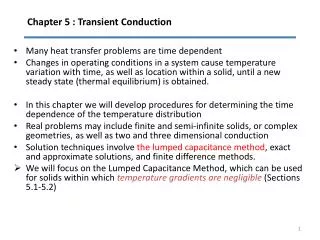
Transient Conduction: The Lumped Capacitance Method
Transient Conduction: The Lumped Capacitance Method. Chapter Five Sections 5.1 thru 5.3. Lecture 9. 1-D Transient Conduction. 1-D conduction in X direction, Not internal heat generation. It can be induced by changes in: surface convection conditions ( ), .

Transient Conduction: The Lumped Capacitance Method
E N D
Presentation Transcript
Transient Conduction:The Lumped Capacitance Method Chapter Five Sections 5.1 thru 5.3 Lecture 9
1-D Transient Conduction 1-D conduction in X direction, Not internal heat generation.
It can be induced by changes in: • surface convection conditions ( ), • surface radiation conditions ( ), Transient Conduction Transient Conduction • A heat transfer process for which the temperature varies with time, as well • as location within a solid. • It is initiated whenever a system experiences a change in operating conditions. • a surface temperature or heat flux, and/or • internal energy generation. • Solution Techniques • The Lumped Capacitance Method • Exact Solutions • The Finite-Difference Method
Consider a general case, which includes convection, radiation and/or an applied heat flux at specified surfaces as well as internal energy generation The Lumped Capacitance Method Lumped Capacitance Method • Based on the assumptionof a spatially uniform temperature distribution • throughout the transient process. Hence, . • Why is the assumption never fully realized in practice? • General Lumped Capacitance • Analysis:
Assuming energy outflow due to convection and radiation and • inflow due to an applied heat flux Lumped Capacitance Method (cont.) • First Law: (5.15) • May h and hr be assumed to be constant throughout the transient process? • How must such an equation be solved?
Negligible Radiation (5.25) Special Case (Negligible Radiation) • Special Cases (Exact Solutions, ) The non-homogeneous differential equation is transformed into a homogeneous equation of the form: Integrating from t = 0to any t and rearranging, To what does the foregoing equation reduce as steady state is approached? How else may the steady-state solution be obtained?
Negligible Radiation and Source Terms (5.2) Special Case (Convection) Note: (5.6) The thermal time constant is defined as (5.7) Thermal Resistance, Rt Lumped Thermal Capacitance, Ct The change in thermal energy storage due to the transient process is (5.8)
Special Case (Radiation) • Negligible Convection and Source Terms Assuming radiation exchange with large surroundings, (5.18) This result necessitates implicit evaluation of T(t).
The Biot Number and Validity of The Lumped Capacitance Method Biot Number • The Biot Number: The first of many dimensionless parameters to be • considered. • Definition: • Physical Interpretation: See Fig. 5.4. • Criterion for Applicability of Lumped Capacitance Method:
Ti t<0, T=Ti Ėout = qconv Liquid Ėst T(t) t≥0 T = T(t) T < Ti The Lumped Capacitance Method
The Lumped Capacitance Method Energy Balance: Ėin + Ėg - Ėout = Ėst -Ėout = -qconv= -hAs(T-T ) = Ėst = Vc(dT/dt) Define: θ ≡ T-T
The Lumped Capacitance Method Thermal Time Constant: τt
The Lumped Capacitance Method Where: Rt isconvection resistance, Ct is lumped thermal capacitance Total energy transfer Q:
T qcond qconv Ts,1 Bi<<1 Ts,2 Bi≈1 Ts,2 Bi>>1 Ts,2 T, h X L Validity of the Lumped Capacitance Method This method is simple and convenient, but it requires Bi < 0.1 T < Ts,2< Ts,1 Under steady-state conditions:
Validity of the Lumped Capacitance Method Biot (Bi) number is the ratio of conduction resistance to convection resistance Characteristic Length Lc≡ V/As Lc= ½ L for plane wall in Fig. 5.4 Lc= r0/2 for long cylinder Lc=r0/3for sphere
Validity of the Lumped Capacitance Method Bi <<1 (Bi < 0.1) Conduction resistance within solid is much less than the resistance to convection across the fluid boundary layer. The T distribution inside the solid is negligible. Lumped capacitance method is valid when Bi<0.1
Validity of the Lumped Capacitance Method Where Fo is Fourier number
Example 5.1 Example 5.1 A thermocouple junction, which may be approximated as a sphere, is to be used to measure the temperature of a gas stream. The convection coefficient is h=400 W/m2·K, k is 20 W/m·k, c=400 J/kg·K, and =8500 kg/m3. Determine the junction diameter needed for the thermocouple to have a time constant of 1 s. If the junction is at 25 ºC and placed in a gas stream that is at 200 ºC, how long will it take for the junction to reach 199 ºC ?
Example 5.1 Known: Thermal properties of the thermocouple junction, time constant. Find: 1. Diameter needed to achieve 1s time constant; 2. Time required to reach 199 ºC in a gas stream at 200 ºC.
D ? Example 5.1 Leads Schematic: Thermocouple Junction Ti=25 ºC T = 200 ºC h=400 W/m2K k=20 W/mK c=400 J/kgK =8500 kg/m3 Gas stream
Example 5.1 Assumptions: • Uniform Temperature inside the junction • Radiation is negligible; • No conduction through the leads; • Constant properties. Analysis: D is unknown, Bi number can’t be determined. But we can assume Bi<0.1, so that Lumped Capacitance method can be applied.
Example 5.1 For sphere, V = πD3/6, As = πD2, Lc =V/As= D/6 Time constant:
Example 5.1 Bi = (hLc/k) =(hD/6k) = 2.35 x 10⁻⁴ <<1 Original assumption (Bi<0.1) is valid, so lumped capacitance method is a good approximation. From Eqn. 5.6
Example 2 (Problem 5.12) A plane wall of a furnace is fabricated from plain carbon steel (k=60 W/mK, ρ=7850kg/m3, c=430J/kgK) and is of thickness L=10 mm. To protect it from the corrosive effects of the furnace combustion gases, one furnace surface of the wall is coated with a thin ceramic film that, for a unit surface area, has a thermal resistance of R”t,f=0.01 m2K/W. the opposite surface is well insulated from the surroundings. At furnace start-up the wall is at initial temperature of Ti=300 K, and the combustion gases at T∞=1300K enter the furnace, providing a convection coefficient h=25 w/m2K at the ceramic film. Assuming the film to have negligible thermal capacitance, how long will it take for the inner surface of the steel to achieve a temperature of Ts,i=1200 K? What is the temp. Ts,o of the exposed surface of the ceramic film at this time?
Problem: Thermal Energy Storage Problem 5.12: Charging a thermal energy storage system consisting of a packed bed of aluminum spheres. Schematic:
Problem: Thermal Energy Storage (cont.) ANALYSIS: To determine whether a lumped capacitance analysis can be used, first compute Bi = h(ro/3) = 75 W/m2∙K (0.0125 m)/150 W/m∙K = 0.006 << 1. From Eq. 5.8, achievement of 90% of the maximum possible thermal energy storage corresponds to < <
Problem: Furnace Start-up Problem 5.22: Heating of coated furnace wall during start-up. Schematic:
Problem: Furnace Start-up (cont.) Hence, with <