Rethinking Steepest Ascent for Multiple Response Applications
330 likes | 509 Views
Rethinking Steepest Ascent for Multiple Response Applications. Robert W. Mee Jihua Xiao University of Tennessee. Outline. Overview of RSM Strategy Steepest Ascent for an Example Efficient Frontier Plots Paths of Improvement (POI) Regions. Sequential RSM Strategy.

Rethinking Steepest Ascent for Multiple Response Applications
E N D
Presentation Transcript
Rethinking Steepest Ascent for Multiple Response Applications Robert W. Mee Jihua Xiao University of Tennessee
Outline • Overview of RSM Strategy • Steepest Ascent for an Example • Efficient Frontier Plots • Paths of Improvement (POI) Regions
Sequential RSM Strategy Box and Wilson (JRSS-B, 1951) • Initial design to estimate linear main effects • Exploration along path of steepest ascent • Repeat step 1 in new optimal location • If main effects are still dominant, repeat step 2; if not, go to step 4 • Augment to complete a 2nd-order design • Optimization based on fitted second-order model
Multiple Responses RSM Literature • Del Castillo (JQT 1996), "Multiresponse Optimization…” • Construct confidence cones for path of steepest ascent (i.e., maximum improvement) for each response • Use very large 1-a for responses of secondary importance, e.g. 99%-99.9% confidence • Use 95%-99% confidence for more critical responses • Identify directions x falling inside every confidence cone • If no such x exists, choose a convex combination of the paths of steepest ascent, giving greater weight for responses that are well estimated • Constrain the solution to reside inside the confidence cones for the most critical responses.
Multiple Responses RSM Literature • Desirability Functions (Derringer and Suich, JQT 1980) • Score each response with a function between 0 and 1. • The geometric mean of the scores is the overall desirability • Recent enhancements use score functions that are “smooth” (i.e., differentiable).
An Example with Multiple Responses • Vindevogel and Sandra (Analytical Chem. 1991) • 25-2 fractional factorial design using micellar electrokinetic chromatography • Higher surfactant levels required to separate two of four esters, but this increases the analysis time • Response variables include: • Resolution for separation of 2nd and 3rd testosterone esters • Time for process, tIV • Four other responses of lesser importance
Reaction Time vs. Reaction Rate • Rate = 1 / Time
Fitted First-Order Models for Resolution and Reaction Rate • Good news: Both models have R2 > 99% • Bad news: Improvement for resolution and rate point in opposite directions • Authors recommend a compromise: • Lower x1 (pH) and x5 (buffer) to increase rate • Lower x2 (SHS%) and x3 (Acet.) and increase x4 (surfactant) to increase resolution.
What about Modeling Desirability? • First-order model for Desirability
What we just tried was a bad idea! • Even when first-order models fit each response well, the desirability function for two or more responses will require a more complicated model • Following an initial two-level design, one cannot model desirability directly. • It is better to maximize desirability based on predicted response values from simple models for each response
Maximizing Predicted Desirability for the Vindevogel and Sandra Example • JMP’s default finds the maximum within a hypercube • This does not identify a useful path for exploration
Confidence Cone for Path of Steepest Ascent (Box and Draper) • Define bb, the angle between least squares estimator b and true coefficient vector b • Pivotal quantity: • Upper confidence bound for sin2bb: • Assuming bb < 90o,
95% Confidence Cone for Paths of Steepest Ascent for Resolution & Rate • 95% Confidence Cones for Paths of Steepest Ascent • Resolution (Y1): bb < 14.4o • Rate (Y2): bb < 32.7o • These confidence cones do not overlap, since the angle between bResolution and bRate is 141.5o! • What compromise is best?
Efficient Frontier Notation • J larger-the-better response variables • First-order model in k factors for each response • Notation • bj: vector of least squares estimates for jth response • Tj: corresponding vector of t statistics for jth response • Convex combinations for two responses • For 0≤c≤1: xC=(1-c)T1 + cT2
Efficient Frontier for Two Responses • Let xN denote a vector that is not a convex combination of T1 and T2 • There exists a convex combination xC, with |xC| = |xN|, such that xC‘bj≥ xN‘bj (j = 1,2) • Proof by contradiction. I.e., suppose not. Then • So one only need consider convex combinations of the paths of steepest ascent.
Efficient Frontier for Resolution and Rate • Predicted Resolution and Rate for x’x=7.49 • Grid lines match Predicted Y @ design center • One quadrant shows gain in both Yj’s Gain!
Efficient Frontier for Resolution and Rate • No change in Rate (Y2): xC=(1-c1)T1 + c1T2 • c1=0.63 • xc = [-0.48, -0.10, -2.68, -0.10, -0.22] @ xc’xc=7.49 • Resolution = 1.76 • Rate = .084
Efficient Frontier for Resolution and Rate • No change in Resolution (Y1): xC=(1-c2)T1 + c2T2 • c2=0.7355 • xc = [-1.39, 0.46, -1.85, -1.22, -0.65] @ xc’xc=7.49 • Resolution = .86 • Rate = .11
Improving Both Responses • If T1’T2 > 0, all convex combinations of T1 and T2 increase the predicted Y for both responses • If T1’T2 < 0, all xc with c1 < c < c2 increase the predicted Y for both responses • For our example, .63 < c < .735 increase predicted Resolution and Rate
Efficient Frontier @ x’x=5versus Factorial Points • Factorial pts. = 8 directions, none on the efficient frontier • What about sampling error?
Attaching Confidence to Improvement • Lower confidence limit for E[Y(x)], given x • Lower confidence limit for change in E[Y(x)], given x where
Efficient Frontier @ x’x=7.49 with 90% Lower Confidence Bound for E(Y)-b0
Paths of Improvement (POI) Region • POI Region = • The POI Region is a cone about the path of steepest ascent, containing all x such that the angle • Using t2,.10 = 1.886, the upper bound for θxb is 86.9o for Resolution, and 83.3o for Rate • For simultaneous (in x) confidence region, replace tdf,a with (kFk,df,a)1/2 or [(k-1)Fk-1,df,a]1/2
Paths of Improvement vs. Path of Steepest Ascent • “Path of Steepest Ascent” b is perpendicular to contours for predicted Y • The path of steepest ascent is not scale invariant • Contours are invariant to the scaling of the factors • Paths of improvement contours are complementary to the confidence cone for steepest ascent path • Assuming bb < 90o, 100(1-a)% confidence cone for steepest ascent • Assuming bb < 90o, 100(1-a)% confidence cone for paths of improvement
Scale Dependence for Path of Steepest Ascent • If the experiment uses a small range for one factor, steepest ascent will neglect that factor • Suppose Y = b0 + X1 + X2 • Experiment 1 • X1: [-2,2] • X2: [-1,1] • Path of S.A.: [4,1] • Experiment 2 • X1: [-1,1] • X2: [-2,2] • Path of S.A.: [1,4] • Contour [1,-1] for both
Complementary Regions As precision improves, the confidence cone for bshrinks, while the paths of improvement region expands toward half of Rk
Common Paths of Improvement • Using predicted values, convex combinations xC=(1-c2)T1 + c2T2 yield improvement in both responses for c1 < c < c2 • For our example, .63 < c < .735 • Using lower confidence bounds, a smaller set of directions yield “certain” improvement in both responses • For our example using t2,.10 = 1.886, we are sure of improvement for .651 < c < .727
Extensions to J > 2 Responses • The efficient frontier for more than two responses is the set of directions x that are a convex combination of all J vectors of steepest ascent • If some directions of steepest ascent are interior to this set, they are not binding • Overlaying contour plots can show the predicted responses for each direction x on the efficient frontier.
Is Simultaneous Improvement Really Possible? • Can we reject Ho: b1b2 = 180o? • An approximate F test based on the difference in SSE for regression of Y2 on X and regression of Y2 on predicted Y1. • For our example, F = 25.45 vs. F4, 2 (p = .04) • Can we construct an upper confidence bound for this angle? • No solution at present • The larger this angle, the further one must extrapolate in these k factors to achieve gain in both responses.