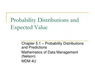
Probability Distributions and Random Variables: Computation, Mean, and Variance
Learn about probability distributions, random variables, expected values, variance, mean, and more. Explore examples and computations for discrete and continuous distributions, including Bernoulli and linear functions.

Probability Distributions and Random Variables: Computation, Mean, and Variance
E N D
Presentation Transcript
Set 4 Probability distribution, expected value, variance
Numerical Random Variables • Unknown quantities • Numerical values associated with outcomes • S = {TTT, TTH, THT, HTT, HHT, HTH, THH, HHH} X = Number of H’s in the outcome • S = { All students in a university} • X = GPA, 0 < x < 4 • Y = Gender, y=0 if male, y=1, if female
Discrete probability distribution • Discrete random variables Y • Countable outcomes • Finite number of outcomes: -1, 0, 2 • Infinite number of outcomes: 0, 1, 2, ... • Also non-integers outcomes: -1.50, 0, 1, 1.5, 2, 2.75 • A probability mass functionf(y)=P(Y=y)directly gives probability of the outcome, y • f(y)tabular, needle (bar) graph, formula • Two properties of f(y): 0 < f(y) < 1 Sf(y) = 1
Continuous probability distribution • Outcomes of random variableYare all numbers in an interval, Y = Income, y > 0; Event A={x: a < y < b } • The points in an interval are not countable • Probability of an outcome in an interval is given by the area under a function f(y) called probability density function P(a < Y < b)
Density function f(y) • Yis continuous • Value of y can be any number in an interval • The points in an interval are not countable • f(y) is the equation of an idealized histogram • Density is always above or on the x-axis, f(y) > 0 • Total area under f(y) = 1 • The probability of the values of y in each interval a<y<b, is given by the area under f(y) • Proportion for any single value of y is zero
Expected value of a random variable • Mean = Expected value of the variable • Discrete distribution E(Y) =Sy f(y) = m • Continuous distribution
Interpretation of the mean • Center of the gravity of the distribution .5 .3 .2 y -1 0 my=.8 2 1.2 -1.8 -.8 0 • Deviations from the mean: y-m • Mean of deviations from the mean is is always zero
Variance of a random variable • Variance = Expected value of the square deviations from the mean Var(Y) = E[(y - m )2 ]=s2 • Discrete distribution Var(Y) =S(y - m )2f(y) = s2 • Continuous distribution • Standard Deviation SD(y) =s
ExampleComputation of mean and variance • Discrete case
Bernoulli Model • Two outcomes • Success (Y=1)withP(Y=1)=p • Failure(Y=0)with P(Y=0)=1-p • Bernoulli distribution • Formulas for mean and variance
Example • 10% of items produced by a machine are defective. • Y= 1, if an item is defective • Y= 0, otherwise • Bernoulli parameter p=.1.
Median,Mean, Mode • Normal density function • Symmetric m Mean = Median = Mode
Median,Mean, Mode • Skewed density function • Right skewed 50% 50% Mode Mean Median
Interpretations • Mean • Weighted average, weight = probability • The balancing point (center of the gravity) • For symmetric distributions, mean = median • Near the long-run average of outcomes of f(y) • Law of large number • An expected value may be an impossible event , so we cannot expect to occur • Variance and Standard deviation • Measures spread of the distribution • Mean and variance are not informative for skewed distributions
Percentiles • Cumulative distribution function CDF(a) = P(Y<a) • CDF(a) = .15, a is the 15th percentile • CDF(a) = .25, a is the 25th percentile (1st quartile, Q1) • CDF(a) = .50, a is the 50th percentile (median) • CDF(a) = .75, a is the 75th percentile (3rd quartile, Q3) • CDF(a) = .95, a is the 95th percentile • Interquartile Range: Q3- Q1
Graph of a discrete CDF • Step function 1 .5 .2 -1 0 2
Discrete CDF • Percentiles may not be unique • 20th percentile is any number in the interval -1<a <0 • Median is any number in the interval 0 <a < 2
Continuous CDF • f(y) is density function • Percentiles are unique • Example: [Normal table gives CDF] • CDF(1.28) = P(Z < 1.28) = .90 .90 Density f(z) .5 CDF F(z) . 90 Height = Fz(1.28) Area =Fz(1.28) 1.28 1.28
Linear function of a random variable • Given a quantitative random variable X • f(x), mx, sx • Another random variable Y is a linear function of X y = a + b x • Mean my = a + b mx • Also true for median, quartiles, percentiles • Variance of the linear function s2y = b2s2x • Standard deviation of the linear function sy = |b|sx • Also true for inter-quartile range
Examples • Given a random variable X with mean and variance • Compute mean, variance and standard deviation of Y = 5 + 2X • Compute mean, variance and standard deviation of V = 5 – 2X