Download
1 / 53
540 likes | 580 Views
Explore simple random sampling, point estimation, and sampling distributions in statistical inference. Understand finite and infinite population sampling methods with examples. Learn about point estimators and sampling error concepts.

E N D
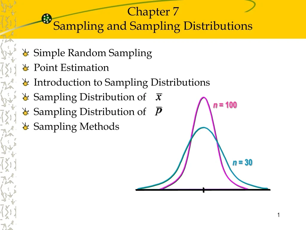
Chapter 7Sampling and Sampling Distributions • Simple Random Sampling • Point Estimation • Introduction to Sampling Distributions • Sampling Distribution of • Sampling Distribution of • Sampling Methods n = 100 n = 30
Statistical Inference • The purpose of statistical inference is to obtain information about a population from information contained in a sample. • A population is the set of all the elements of interest. • A sample is a subset of the population. • The sample results provide only estimates of the values of the population characteristics. • A parameter is a numerical characteristic of a population. • With proper sampling methods, the sample results will provide “good” estimates of the population characteristics.
Simple Random Sampling • Finite Population • A simple random sample from a finite population of size N is a sample selected such that each possible sample of size n has the same probability of being selected. • Replacing each sampled element before selecting subsequent elements is called sampling with replacement.
Simple Random Sampling • Finite Population • Sampling without replacement is the procedure used most often. • In large sampling projects, computer-generated random numbers are often used to automate the sample selection process.
Simple Random Sampling • Infinite Population • A simple random sample from an infinite population is a sample selected such that the following conditions are satisfied. • Each element selected comes from the same population. • Each element is selected independently.
Simple Random Sampling • Infinite Population • The population is usually considered infinite if it involves an ongoing process that makes listing or counting every element impossible. • The random number selection procedure cannot be used for infinite populations.
Point Estimation • In point estimation we use the data from the sample to compute a value of a sample statistic that serves as an estimate of a population parameter. • We refer to as the point estimator of the population mean . • s is the point estimator of the population standard deviation . • is the point estimator of the population proportion p.
Point Estimation • When the expected value of a point estimator is equal to the population parameter, the point estimator is said to be unbiased.
Sampling Error • The absolute difference between an unbiased point estimate and the corresponding population parameter is called the sampling error. • Sampling error is the result of using a subset of the population (the sample), and not the entire population to develop estimates. • The sampling errors are: for sample mean for sample standard deviation for sample proportion
Example: St. Andrew’s St. Andrew’s College receives 900 applications annually from prospective students. The application forms contain a variety of information including the individual’s scholastic aptitude test (SAT) score and whether or not the individual desires on-campus housing.
Example: St. Andrew’s The director of admissions would like to know the following information: • the average SAT score for the applicants, and • the proportion of applicants that want to live on campus.
Example: St. Andrew’s We will now look at three alternatives for obtaining the desired information. • Conducting a census of the entire 900 applicants • Selecting a sample of 30 applicants, using a random number table • Selecting a sample of 30 applicants, using computer-generated random numbers
Example: St. Andrew’s • Taking a Census of the 900 Applicants • SAT Scores • Population Mean • Population Standard Deviation
Example: St. Andrew’s • Taking a Census of the 900 Applicants • Applicants Wanting On-Campus Housing • Population Proportion
Example: St. Andrew’s • Take a Sample of 30 Applicants Using a Random Number Table Since the finite population has 900 elements, we will need 3-digit random numbers to randomly select applicants numbered from 1 to 900. We will use the last three digits of the 5-digit random numbers in the third column of the textbook’s random number table (Table 7.1, p. 259).
Example: St. Andrew’s • Take a Sample of 30 Applicants Using a Random Number Table The numbers we draw will be the numbers of the applicants we will sample unless • the random number is greater than 900 or • the random number has already been used. We will continue to draw random numbers until we have selected 30 applicants for our sample.
Example: St. Andrew’s • Use of Random Numbers for Sampling 3-Digit Applicant Random NumberIncluded in Sample 744 No. 744 436 No. 436 865 No. 865 790 No. 790 835 No. 835 902 Number exceeds 900 190 No. 190 436 Number already used etc. etc.
Example: St. Andrew’s • Sample Data Random No.NumberApplicantSAT ScoreOn-Campus 1 744 Connie Reyman 1025 Yes 2 436 William Fox 950 Yes 3 865 Fabian Avante 1090 No 4 790 Eric Paxton 1120 Yes 5 835 Winona Wheeler 1015 No . . . . . 30 685 Kevin Cossack 965 No
Example: St. Andrew’s • Take a Sample of 30 Applicants Using Computer-Generated Random Numbers • Excel provides a function for generating random numbers in its worksheet. • 900 random numbers are generated, one for each applicant in the population. • Then we choose the 30 applicants corresponding to the 30 smallest random numbers as our sample. • Each of the 900 applicants have the same probability of being included.
Using Excel to Selecta Simple Random Sample • Formula Worksheet Note: Rows 10-901 are not shown.
Using Excel to Selecta Simple Random Sample • Value Worksheet Note: Rows 10-901 are not shown.
Using Excel to Selecta Simple Random Sample • Value Worksheet (Sorted) Note: Rows 10-901 are not shown.
Example: St. Andrew’s • Point Estimates • as Point Estimator of • s as Point Estimator of • as Point Estimator of p
Example: St. Andrew’s • Point Estimates Note:Different random numbers would have identified a different sample which would have resulted in different point estimates.
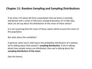
Sampling Distribution of The value of is used to make inferences about the value of m. The sample data provide a value for the sample mean . • Process of Statistical Inference Population with mean m = ? A simple random sample of n elements is selected from the population.
Sampling Distribution of • The sampling distribution of is the probability distribution of all possible values of the sample mean . • Expected Value of E( ) = where: = the population mean • What does this imply? • The sample mean (from a simple random sample) is an unbiased estimator of population mean.
Sampling Distribution of • : Standard Deviation of • referred to as the standard error of the mean. Finite Population Infinite Population • A finite population is treated as being infinite if n/N< .05. • is the finite correction factor.
Sampling Distribution of • If we use a large (n> 30) simple random sample, the central limit theorem enables us to conclude that the sampling distribution of can be approximated by a normal probability distribution. • When the simple random sample is small (n < 30), the sampling distribution of can be considered normal only if we assume the population has a normal probability distribution.
Example: St. Andrew’s • Sampling Distribution of for the SAT Scores
Example: St. Andrew’s • Sampling Distribution of for the SAT Scores What is the probability that a simple random sample of 30 applicants will provide an estimate of the population mean SAT score that is within plus or minus 10 of the actual population mean ? In other words, what is the probability that will be between 980 and 1000?
Example: St. Andrew’s • Sampling Distribution of for the SAT Scores Sampling distribution of Area = ? 980 990 1000
Example: St. Andrew’s • Sampling Distribution of for the SAT Scores Using the standard normal probability table with z = 10/14.6= .68, we have area = (.2517)(2) = .5034 The probability is .5034 that the sample mean will be within +/-10 of the actual population mean.
Example: St. Andrew’s Sampling distribution of Area = 2(.2517) = .5034 980 990 1000 • Sampling Distribution of for the SAT Scores
Sampling Distribution of • The sampling distribution of is the probability distribution of all possible values of the sample proportion . • Expected Value of where: p = the population proportion
Sampling Distribution of • Standard Deviation of Finite Population Infinite Population • is referred to as the standard error of the proportion.
Sampling Distribution of • The sampling distribution of can be approximated by a normal probability distribution whenever the sample size is large. • The sample size is considered large whenever these conditions are satisfied: np> 5 and n(1 – p) > 5
Sampling Distribution of • For values of p near .50, sample sizes as small as 10 permit a normal approximation. • With very small (approaching 0) or large (approaching 1) values of p, much larger samples are needed.
Example: St. Andrew’s • Sampling Distribution of for Applicants Desiring On-campus Housing The normal probability distribution is an acceptable approximation because: np = 30(.72) = 21.6 > 5 and n(1 - p) = 30(.28) = 8.4 > 5.
Example: St. Andrew’s • Sampling Distribution of for Applicants Desiring On-campus Housing
Example: St. Andrew’s • Sampling Distribution of for Applicants Desiring On-campus Housing What is the probability that a simple random sample of 30 applicants will provide an estimate of the population proportion of applicants desiring on-campus housing that is within plus or minus .05 of the actual population proportion? In other words, what is the probability that will be between .67 and .77?
Example: St. Andrew’s • Sampling Distribution of for Applicants Desiring On-campus Housing Sampling distribution of Area = ? 0.77 0.67 0.72
Example: St. Andrew’s • Sampling Distribution of for Applicants Desiring On-campus Housing For z = .05/.082 = .61, the area = (.2291)(2) = .4582. The probability is .4582 that the sample proportion will be within +/-.05 of the actual population proportion.
Example: St. Andrew’s • Sampling Distribution of for In-State Residents Sampling distribution of Area = 2(.2291) = .4582 0.77 0.67 0.72
Sampling Methods • Stratified Random Sampling • Cluster Sampling • Systematic Sampling • Convenience Sampling • Judgment Sampling
Stratified Random Sampling • The population is first divided into groups of elements called strata. • Each element in the population belongs to one and only one stratum. • Best results are obtained when the elements within each stratum are as much alike as possible (i.e. homogeneous group). • A simple random sample is taken from each stratum. • Example: The basis for forming the strata might be department, location, age, industry type, etc.
Stratified Random Sampling • Advantage: If strata are homogeneous, this method is as “precise” as simple random sampling but with a smaller total sample size. • Formulas are available for combining the stratum sample results into one population parameter estimate.
Cluster Sampling • The population is first divided into separate groups of elements called clusters. • Ideally, each cluster is a representative small-scale version of the population (i.e. heterogeneous group). • A simple random sample of the clusters is then taken. • All elements within each sampled (chosen) cluster form the sample. • Example: A primary application is area sampling, where clusters are city blocks or other well-defined areas. … continued
Cluster Sampling • Advantage: The close proximity of elements can be cost effective (I.e. many sample observations can be obtained in a short time). • Disadvantage: This method generally requires a larger total sample size than simple or stratified random sampling.
Systematic Sampling • If a sample size of n is desired from a population containing N elements, we might sample one element for every N/n elements in the population. • We randomly select one of the first N/n elements from the population list. • We then select every N/nth element that follows in the population list. • This method has the properties of a simple random sample, especially if the list of the population elements is a random ordering. … continued
Systematic Sampling • Advantage: The sample usually will be easier to identify than it would be if simple random sampling were used. • Example: Selecting every 100th listing in a telephone book after the first randomly selected listing.