Chapter 7 Sampling and Sampling Distributions

1. Sampling Distribution of Chapter 7Sampling and Sampling Distributions • Simple Random Sampling • Point Estimation • Introduction to Sampling Distributions

2. Example: St. Andrew’s St. Andrew’s College receives 900 applications annually from prospective students. The application form contains a variety of information including the individual’s scholastic aptitude test (SAT) score and whether or not the individual desires on-campus housing.

3. Example: St. Andrew’s The director of admissions would like to know the following information: • the average SAT score for the 900 applicants, and • the proportion of applicants that want to live on campus.

4. Example: St. Andrew’s We will now look at three alternatives for obtaining the desired information. • Conducting a census of the entire 900 applicants • Selecting a sample of 30 applicants, using a random number table • Selecting a sample of 30 applicants, using Excel

5. Conducting a Census • If the relevant data for the entire 900 applicants were in the college’s database, the population parameters of interest could be calculated using the formulas presented in Chapter 3. • We will assume for the moment that conducting a census is practical in this example.

6. Conducting a Census • Population Mean SAT Score • Population Standard Deviation for SAT Score • Population Proportion Wanting On-Campus Housing

7. as Point Estimator of  • as Point Estimator of p Point Estimation • s as Point Estimator of  Note:Different random numbers would have identified a different sample which would have resulted in different point estimates.

8. = Sample mean SAT score = Sample pro- portion wanting campus housing Summary of Point Estimates Obtained from a Simple Random Sample Population Parameter Parameter Value Point Estimator Point Estimate m = Population mean SAT score 990 997 80 s = Sample std. deviation for SAT score 75.2 s = Population std. deviation for SAT score .72 .68 p = Population pro- portion wanting campus housing

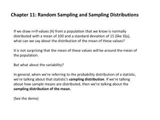
9. Sampling Distribution of The value of is used to make inferences about the value of m. The sample data provide a value for the sample mean . • Process of Statistical Inference A simple random sample of n elements is selected from the population. Population with mean m = ?

10. Sampling Distribution of Expected Value of E( ) =  The sampling distribution of is the probability distribution of all possible values of the sample mean . where:  = the population mean

11. Sampling Distribution of Standard Deviation of • is the finite correction factor. • is referred to as the standard error of the • mean. Finite Population Infinite Population • A finite population is treated as being • infinite if n/N< .05.

12. Form of the Sampling Distribution of If we use a large (n> 30) simple random sample, the central limit theorem enables us to conclude that the sampling distribution of can be approximated by a normal distribution. When the simple random sample is small (n < 30), the sampling distribution of can be considered normal only if we assume the population has a normal distribution.

13. Sampling Distribution of for SAT Scores Sampling Distribution of

14. Sampling Distribution of for SAT Scores With a mean SAT score of 990 and a standard deviation of 80, what is the probability that a simple random sample of 30 applicants will provide an estimate of the population mean SAT score that is within +/-10 of the actual population mean  ? In other words, what is the probability that will be between 980 and 1000?

15. Sampling Distribution of for SAT Scores Step 1: Calculate the z-value at the upper endpoint of the interval. z = (1000 - 990)/14.6= .68 Step 2: Find the area under the curve between the mean and the upper endpoint. .2517

16. Sampling Distribution of for SAT Scores Probabilities for the Standard Normal Distribution

17. Sampling Distribution of for SAT Scores Sampling Distribution of Area = .2517 990 1000

18. Sampling Distribution of for SAT Scores Step 3: Calculate the z-value at the lower endpoint of the interval. z = (980 - 990)/14.6= - .68 Step 4: Find the area under the curve between the mean and the lower endpoint. = .2517

19. Sampling Distribution of for SAT Scores Sampling Distribution of Area = .2517 980 990

20. Sampling Distribution of for SAT Scores Sampling Distribution of Area = .2517 Area = .2517 980 990 1000

21. Sampling Distribution of for SAT Scores P(980 << 1000) = .5034 Step 5: Calculate the area under the curve between the lower and upper endpoints of the interval. P(-.68 <z< .68) = = .2517 + .2517 = .5034 The probability that the sample mean SAT score will be between 980 and 1000 is:

22. Sampling Distribution of for SAT Scores Sampling Distribution of Area = .5034 980 990 1000

23. Relationship Between the Sample Size and the Sampling Distribution of • E( ) = m regardless of the sample size. In our example, E( ) remains at 990. • Whenever the sample size is increased, the standard error of the mean is decreased. With the increase in the sample size to n = 100, the standard error of the mean is decreased to: • Suppose we select a simple random sample of 100 applicants instead of the 30 originally considered.

24. Relationship Between the Sample Size and the Sampling Distribution of With n = 100, With n = 30,

25. Relationship Between the Sample Size and the Sampling Distribution of • Recall that when n = 30, P(980 << 1000) = .5034. • We follow the same steps to solve for P(980 << 1000) when n = 100 as we showed earlier when n = 30. • Now, with n = 100, P(980 << 1000) = .7888. • Because the sampling distribution with n = 100 has a smaller standard error, the values of have less variability and tend to be closer to the population mean than the values of with n = 30.

26. Relationship Between the Sample Size and the Sampling Distribution of Sampling Distribution of Area = .7888 980 990 1000

27. Sampling Distribution of Chapter 7 Sampling and Sampling Distributions • Other Sampling Methods

28. Sampling Distribution of The sample data provide a value for the sample proportion . The value of is used to make inferences about the value of p. • Making Inferences about a Population Proportion A simple random sample of n elements is selected from the population. Population with proportion p = ?

29. Sampling Distribution of Expected Value of The sampling distribution of is the probability distribution of all possible values of the sample proportion . where: p = the population proportion

30. Sampling Distribution of Standard Deviation of is referred to as the standard error of the proportion. Finite Population Infinite Population • A finite population is treated as being • infinite if n/N< .05.

31. Sampling Distribution of • Example: St. Andrew’s College Recall that 72% of the prospective students applying to St. Andrew’s College desire on-campus housing. What is the probability that a simple random sample of 30 applicants will provide an estimate of the population proportion of applicant desiring on-campus housing that is within plus or minus .05 of the actual population proportion?

32. Sampling Distribution of Sampling Distribution of

33. Sampling Distribution of Step 1: Calculate the z-value at the upper endpoint of the interval. z = (.77 - .72)/.082 = .61 Step 2: Find the area under the curve between the mean and upper endpoint. .2291

34. Sampling Distribution of Probabilities for the Standard Normal Distribution

35. Sampling Distribution of Sampling Distribution of Area = .2291 .72 .77

36. Sampling Distribution of Step 3: Calculate the z-value at the lower endpoint of the interval. z = (.67 - .72)/.082 = - .61 Step 4: Find the area under the curve between the mean and the lower endpoint. .2291

37. Sampling Distribution of Sampling Distribution of Area = .2291 .67 .72

38. Sampling Distribution of P(.67 << .77) = .4582 Step 5: Calculate the area under the curve between the lower and upper endpoints of the interval. P(-.61 <z< .61) = = .2291 + .2291 = .4582 The probability that the sample proportion of applicants wanting on-campus housing will be within +/-.05 of the actual population proportion :

39. Sampling Distribution of Sampling Distribution of Area = .4582 .67 .72 .77

40. Other Sampling Methods • Stratified Random Sampling • Cluster Sampling • Systematic Sampling • Convenience Sampling • Judgment Sampling

41. Stratified Random Sampling The population is first divided into groups of elements called strata. Each element in the population belongs to one and only one stratum. Best results are obtained when the elements within each stratum are as much alike as possible (i.e. a homogeneous group).

42. Stratified Random Sampling A simple random sample is taken from each stratum. Formulas are available for combining the stratum sample results into one population parameter estimate. Advantage: If strata are homogeneous, this method is as “precise” as simple random sampling but with a smaller total sample size. Example: The basis for forming the strata might be department, location, age, industry type, and so on.

43. Cluster Sampling The population is first divided into separate groups of elements called clusters. Ideally, each cluster is a representative small-scale version of the population (i.e. heterogeneous group). A simple random sample of the clusters is then taken. All elements within each sampled (chosen) cluster form the sample.

44. Cluster Sampling Example: A primary application is area sampling, where clusters are city blocks or other well-defined areas. Advantage: The close proximity of elements can be cost effective (i.e. many sample observations can be obtained in a short time). Disadvantage: This method generally requires a larger total sample size than simple or stratified random sampling.

45. Systematic Sampling If a sample size of n is desired from a population containing N elements, we might sample one element for every n/N elements in the population. We randomly select one of the first n/N elements from the population list. We then select every n/Nth element that follows in the population list.

46. Systematic Sampling This method has the properties of a simple random sample, especially if the list of the population elements is a random ordering. Advantage: The sample usually will be easier to identify than it would be if simple random sampling were used. Example: Selecting every 100th listing in a telephone book after the first randomly selected listing

47. Convenience Sampling It is a nonprobability sampling technique. Items are included in the sample without known probabilities of being selected. The sample is identified primarily by convenience. Example: A professor conducting research might use student volunteers to constitute a sample.

48. Convenience Sampling Advantage: Sample selection and data collection are relatively easy. Disadvantage: It is impossible to determine how representative of the population the sample is.

49. Judgment Sampling The person most knowledgeable on the subject of the study selects elements of the population that he or she feels are most representative of the population. It is a nonprobability sampling technique. Example: A reporter might sample three or four senators, judging them as reflecting the general opinion of the senate.

50. Judgment Sampling Advantage: It is a relatively easy way of selecting a sample. Disadvantage: The quality of the sample results depends on the judgment of the person selecting the sample.