Download
1 / 32
340 likes | 513 Views
SuperScalar Design Prime. Zhao Zhang CprE 381, Computer Organization and Assembly-Level Programming, Fall 2012 Original slides from CprE 581, Advanced Computer Architecture. History Superscalar Design. First appearance in 1960s Scoreboarding Tomasulo Algorithm

E N D
SuperScalar Design Prime Zhao Zhang CprE 381, Computer Organization and Assembly-Level Programming, Fall 2012 Original slides from CprE 581, Advanced Computer Architecture
History Superscalar Design First appearance in 1960s • Scoreboarding • Tomasulo Algorithm Popular use since 1990s • SGI MIPS processors • Sun UltraSPARC • Dec Alpha 21x64 series • Intel/AMD processors Now appearing in embedded processors • Cortex-A9: Two-way, limited out-of-order • Certex-A15: Three-way, close to Intel/AMD design
Why Superscalar Get more performance than scalar pipeline Superscalar Techniques: Deep pipeline Multi-issue Branch prediction Register renaming Out-of-order Execution Speculative Execution Memory disambiguation
Code Example for (i = 0; i < 1000; i++) X[i] = X[i] + b; ; loop body, initialization not shown ; R4: &X[i], R5: (X+1000)*4, R6: b Loop: LW R8, R4($0) ; load X[i], R4 stores X ADD R8, R8, R6 ; X[i] = X[i] + b SW R8, R4($0) ; store X[i] ADDI R4, R4, 4 ; next element SLT R9, R4, R5 ; R9 = (R4 < R5) BNE R9, R0, loop ; end of loop?
Frontend and Backend Frontend: In-order fetch, decode, and rename Backend: Out-of-order issue, execute/writeback, in-order commit Frontend may send “junk” instructions to the backend • Junk instructions occur with branch mis-prediction or exceptions • Design goal: Minimize the percentage of “junk” instructions Backend must be able to detect and handle “junk” instructions • Flush junk instructions upon detetion • In-order commit (retire) so that junk instructions won’t affect the “architectural state” • Dozens of cycles likely for handling a branch mis-prediction
Frontend and Backend Frontend Backend “Cortex-A9 Processor Microarchitecture”, slide 6
The Multi-Issue Factor Multi-issue affects all pipeline stages: In the same cycle, • N inst. are fetched: Usually from one I-cache block • N inst. are decoded: Multiple decoders • N inst. are renamed: Multi-ported renaming table, detecting intra-group dependence In the backend • Up to N inst. are scheduled: Multi-ported queue with broadcast • N inst. read register file: Multi-ported register file • M inst. are executed at functional units: Multiple functional units • N inst. writes back register values: multi-ported register file • N inst. are committed: Multi-banked reorder buffer, also involves rename table Note: “N” is not necessary the same value across pipeline stages
Frontend: Branch Prediction Branch prediction is critical to reducing “junk” instructions With “disaster” branch prediction performance: SPECint programs have on average ~15% branches • Every 100 instructions contain 15 branches • Assume 10% mis-prediction => 1.5 branch mis-predictions • Assume 20-cycle mis-prediction penalty => 30 lost cycles • Assume IPC=3.0 => 33.3 cycles for execution 100 inst • 90% loss for the 10% mis-prediction • Mis-prediction penalty is workload-dependent, and can be significantly longer than 20 cycles good inst good inst good inst
Frontend: Branch Prediction Branch prediction is made every cycle • Otherwise, instruction flow stops • It’s done in parallel with instruction fetch The backend sends back feedback about past predictions Single cycle loop Pred-PC Inst. Cache Target, branch, and return addr.predictors INST Feedback from the backend
Frontend: Branch Prediction Three components in simple design Branch Target Buffer (BTB): What’s the branch target? Branch History Table (BHT): Is the branch taken or not? Return Address Stack (RAS) • Function return is a special type of branch instruction • There are multiple valid branch targets for the return How BTB and BHT works in general • Bet the same patterns will repeat • Use only PC and past branch outcome history in the prediction
Branch PC Predicted PC Frontend: Branch Prediction Branch Target Buffer with combined Branch History Table PC of instruction FETCH =? Extra prediction state Bits (see later) Yes: instruction is branch and use predicted PC as next PC No: branch not predicted, proceed normally (Next PC = PC+4) From slides of CprE 581 Computer Systems Architecture
-- -- 0 -- -- 0 -- -- 0 -- -- 0 -- -- 0 -- -- 0 Branch PC Predicted PC Frontend: Branch Prediction First time fetching at BNE: Predicted as Not Taken Loop: LW R8, R4($0) ; load X[i], R4 stores X ADD R8, R8, R6 ; X[i] = X[i] + b SW R8, R4($0) ; store X[i] ADDI R4, R4, 4 ; next element SLT R9, R4, R5 ; end of array? BNE R9, R0, loop => mis-prediction on 1st fetch LW ADD SW ADDI STL BNE => NT, right => NT, right => NT, right => NT, right => NT, right => NT, WRONG
-- -- 0 -- -- 0 -- -- 0 -- -- 0 -- -- 0 BNE-PC LW-PC 1 Branch PC Predicted PC Frontend: Branch Prediction What happen after the mis-prediction • The frontend starts fetch junk instructions, probably in dozens • The backend detects the mis-prediction, flush backend pipeline, notifies the frontend about the mis-predicted branch • The frontend updates the BTB/BHT, filling in BNE-PC and LW-PC, change prediction state bit • The frontend restarts fetching from LW-PC LW ADD SW ADDI STL BNE
-- -- 0 -- -- 0 -- -- 0 -- -- 0 -- -- 0 BNE-PC LW-PC 1 Branch PC Predicted PC Frontend: Branch Prediction 2nd time fetching at BNE: Predicted as Taken, jump to LW-PC Loop: LW R8, R4($0) ; load X[i], R4 stores X ADD R8, R8, R6 ; X[i] = X[i] + b SW R8, R4($0) ; store X[i] ADDI R4, R4, 4 ; next element SLT R9, R4, R5 ; end of array? => BNE R9, R0, loop ; LW ADD SW ADDI STL BNE => NT, right => NT, right => NT, right => NT, right => NT, right => Taken, RIGHT
-- -- 0 -- -- 0 -- -- 0 -- -- 0 -- -- 0 BNE-PC LW-PC 0 Branch PC Predicted PC Frontend: Branch Prediction Last time fetching at BNE-PC, predicted as Taken • It’s wrong because the loop will exit This time, the prediction state bit is changed to 0 • Next time the prediction outcome on BNE-PC is Not Taken LW ADD SW ADDI STL BNE
Branch Prediction State Bit General Form 1. Access 2. Predict Output T/NT state PC 3. Feedback T/NT 1-bit prediction Feedback T NT NT 1 0 Predict NotTaken Predict Taken T From CprE 581, Computer Systems Architecture
Branch History Table Branch direction prediction is usually more challenging • BHT can be separated from BTB (often the case) • 2-bit or 3-bit state are usually used • BHT can be organized in two levels to predict on correlation between branches • BHT can have sophisticated organizations to further improve accuracy Return Address Stack: Work on return instructions, simple and effective (not to be discussed more)
Frontend: Register Renaming Consider two loop iterations: Conflict on register usage, cannot be executed in parallel, but they are mostly parallel LW R8, R4($0) ; load X[i], R4 stores X ADD R8, R8, R6 ; X[i] = X[i] + b SW R8, R4($0) ; store X[i] ADDI R4, R4, 4 ; next element SLT R9, R4, R5 ; end of array? BNE R9, R0, loop ; LW R8, R4($0) ; load X[i], R4 stores X ADD R8, R8, R6 ; X[i] = X[i] + b SW R8, R4($0) ; store X[i] ADDI R4, R4, 4 ; next element SLT R9, R4, R5 ; end of array? BNE R9, R0, loop ;
Frontend: Register Renaming Rename architectural registers to physical registers, remove false dependence and keep true dep. LWP32, P4($0) ; load X[i], R4 stores X ADD P33, P32, P6 ; X[i] = X[i] + b SW P33, P4($0) ; store X[i] ADDI P34, P4, 4 ; next element SLT P35, P34, P5 ; end of array? BNE P35, P0, loop ; LWP36, P34($0) ; load X[i], R4 stores X ADD P37, P36, P6 ; X[i] = X[i] + b SW P37, P34($0) ; store X[i] ADDI P38, P34, 4 ; next element SLT P38, P38, P5 ; end of array? BNE R38, p0, loop ;
Frontend: Register Renaming How the design works: • There is a register mapping table that maps architecture register to physical register • There is a queue of free physical register • Every instruction with output register is assigned with an unused, free physical register • Another mapping table is used to recover from mis-predicted path • There are a number of design variants in real processors
Frontend: Register Renaming The roles of register renaming: • Remove register name dependence, keep true data dependence, so that more instructions can be safely reordered • Help backend implement speculative execution, as no junk instructions cannot affect the input of good instructions • A younger instruction writes to newly assigned physical register, so it cannot affect the input of old instructions • A good instruction is always older than any junk instruction
Backend: Out-Of-Order Scheduling Common Design: Issue Queue Op busy? dst src1 ready? src2 ready? ROB LSQ 1 yes 0x0 yes 1 LW yes P32 P4 - no P6 yes 2 ADD yes P33 P32 2 no P4 yes 3 SW yes -- P33 - yes 0x4 yes 4 ADDI yes P34 P4 - no P5 yes 5 SLT yes P35 P34 - no P0 yes 6 BNE yes -- P35
Backend: Out-Of-Order Scheduling Schedule: Select ready instructions, broadcast their tag (dst) to all other instructions for matching Op busy? dst src1 ready? src2 ready? ROB LSQ 1 yes 0x0 yes 1 LW yes P32 P4 - no P6 yes 3 ADD yes P33 P32 2 no P4 yes 2 SW yes -- P33 - yes 0x4 yes 4 ADDI yes P34 P4 - no P5 yes 5 SLT yes P35 P34 - no P0 yes 6 BNE yes -- P35
Backend: Out-Of-Order Scheduling After LW and ADDI are issued, assume no new instructions Op busy? dst src1 ready? src2 ready? ROB LSQ -- -- -- -- -- -- no -- -- - yes P6 yes 2 ADD yes P33 P32 2 no P4 yes 3 SW yes -- P33 - -- -- -- -- -- -- -- -- - yes P5 yes 5 SLT yes P35 P34 - no P0 yes 6 BNE yes -- P35
Backend: Out-Of-Order Scheduling After ADD and SLT are issued, assume no new instructions Op busy? dst src1 ready? src2 ready? ROB LSQ -- -- -- -- -- -- no -- -- - -- -- -- -- -- no -- -- 2 yes P4 yes 2 SW yes -- P33 - -- -- -- -- -- -- -- -- - -- -- -- -- -- -- -- -- - yes P0 yes 6 BNE yes -- P35
Backend: Out-Of-Order Scheduling How the design works • Instructions are sent to the issue queue after renaming • A select logic chooses up to N instructions, all dependence free, to be executed • The tag of the selected instructions are broadcast to all other queue entries • A wakeup logic clears the dependence of other instructions on the selected instructions Two major design variants: Issue Queue vs. Reservation Station
Backend: Register Read, Data Forwarding and Writeback Note: In reservation-station design, register-read happens before instruction scheduling Issue Queue Issue (scheduling) Register File Reg-Read Forwarding Network Execute Load Store Int Mult Div Other Writeback
Reorder Buffer and In-Order Commit head tail head tail … … freed head tail … allocated
Program Counter Branch or L/W? Dest arch reg Destphyreg Exceptions? Ready? Reorder Buffer Reorder Buffer and In-Order Commit Instructions enter and leave ROB in program order “Architectural Register State” changes in program order Junk instructions may produce values, but their values never appear in the “Architectural Register State” • Junk instructions will be flushed upon detection
Recall the Renaming Example Consider two loop iterations: Rename architectural registers to physical registers, remove false dependence and keep true dep. LWP32, P4($0) ; load X[i], R4 stores X ADD P33, P32, P6 ; X[i] = X[i] + b SW P33, P4($0) ; store X[i] ADDI P34, P4, 4 ; next element SLT P35, P34, P5 ; end of array? BNE P35, P0, loop ; LWP36, P34($0) ; load X[i], R4 stores X ADD P37, P36, P6 ; X[i] = X[i] + b SW P37, P34($0) ; store X[i] ADDI P38, P34, 4 ; next element SLT P38, P38, P5 ; end of array? BNE R38, p0, loop ;
Architectural Register State architectural register mapping LW R8, R4($0) ADD R8, R8, R6 SW R8, R4($0) ADDI R4, R4, 4 SLT R9, R4, R5 BNE R9, R0, loop LW R8, R4($0) ADD R8, R8, R6 SW R8, R4($0) ADDI R4, R4, 4 SLT R9, R4, R5 BNE R9, R0, loop speculative register mapping architectural register mapping speculative register mapping Mis-predicted path architectural register mapping speculative register mapping
Summary What we have learned • In-order frontend vs. out-of-order backend • Branch prediction to keep instruction flow • Register renaming to remove name dependence and support speculative execution • Out-of-order scheduling with issue queue • In-order commit with re-order buffer What we haven’t learned yet • Memory disambiguation using load/queue and store queue • Detail in complex real processors