Download

1 / 36
380 likes | 813 Views
Multivariate Analysis of Variance (MANOVA). Outline. Purpose and logic : page 3 Hypothesis testing : page 6 Computations: page 11 F -Ratios: page 25 Assumptions and noncentrality : page 35. MANOVA. When ?

E N D
Outline • Purpose and logic : page 3 • Hypothesis testing :page 6 • Computations:page 11 • F-Ratios: page 25 • Assumptions and noncentrality : page 35
MANOVA • When ? • When a research design contains two or more dependent variables we could perform multiple univariate tests or one multivariate test • Why ? • MANOVA does not have the problem of inflated overall type I error rate (a) • Univariate tests ignore the correlations among the variables • Multivariate tests are more powerful than multiple univariate tests • Assumptions • Multivariate normality • Absence of outliers • Homogeneity of variance-covariance matrices • Linearity • Absence of multicollinearity
MANOVA • If the independent variables are discrete and the dependant variables are continuous we will performed a MANOVA From MANOVA where, m = grand mean, a = treatment effect 1, b = treatment effect 2, ab = interaction, e = error To GLM where,
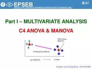
MANOVA • The general idea behind MANOVA is the same as previously. We want to find a ratio between explained variability over unexplained variability (error) a = treatment effect 1 (rows; r = 2) b = treatment effect 2 (columns; c = 3) ni = 4 N = r*c*ni=24 q = number of DV = 2 (WeightLoss, Time) • Example
Analysis of Variance (ANOVA) • Hypothesis • Are the drug mean vectors equal? • Are the sex mean vectors equal? • Do some drugs interact with sex to produce inordinately high or low weight decrements?
Analysis of Variance (ANOVA) Using the GLM approach through a coding matrix
Analysis of Variance (ANOVA) Then, for each subject we associate its corresponding group coding.
Canonical correlation matrix • R is obtained by:
Error Matrix (E) • In ANOVA, the error was defined as e = (1-R2)Scc • This is a special case of the MANOVA error matrix E
Hypothesis variation matrix • The total variation is the sum of the various hypothesis variation add to the error variation, i.e. T=E+H+H+H. • Each matrix H is obtained by • Where i{, , } • The full model is omitted when performing hypothesis testing • (We start by testing the interaction, then the main effects, etc.)
Hypothesis variation matrix =Mab • Interaction
Hypothesis variation matrix • Interaction
Here is the catch! • In univariate, the statistics is based on the F-ratio distribution • However, in MANOVA there is no unique statistic. Four statistics are commonly used: Hotelling-Lawley trace (HL), Pillai-Bartlett trace (PB), Wilk`s likelihood ratio (W) and Roy’s largest root (RLR).
Hotelling-Lawley trace (HL) • The HL statistic is defined as • where s = min(dfi, q), i represents the tested effect (i{a, b, ab}), dfi is the degree of freedom associated with the hypothesis under investigation (a, b or ab) and lk is kth eigenvalue extracted from HiE-1.
Hotelling-Lawley trace (HL) • Interaction • Extracted eigenvalues
Hotelling-Lawley trace (HL) • Interaction Trace • dfab = (r-1)(c-1)=(2-1)(3-1) = 2 • s = min(dfab, q) = min(2, 2) = 2
Pillai-Bartlett trace (PB) • The PB statistic is defined as • where s = min(dfi, q), i represents the tested effect (i{a, b, ab}), dfi is the degree of freedom associated with the hypothesis under investigation (a, b or ab) and lk is kth eigenvalue extracted from HiE-1.
Pillai-Bartlett trace (PB) • Interaction • dfab = (r-1)(c-1)=(2-1)(3-1) = 2 • s = min(dfab, q) = min(2, 2) = 2
Wilk’slikelihood ratio (W) • The W statistic is defined as • where s = min(dfi, q), i represents the tested effect (i{a, b, ab}), dfi is the degree of freedom associated with the hypothesis under investigation (a, b or ab), lk is kth eigenvalue extracted from HiE-1 and |E| (as well as |E+Hi|) is the determinant.
Wilk’slikelihood ratio (W) • Interaction • dfab = (r-1)(c-1)=(2-1)(3-1) = 2 • s = min(dfab, q) = min(2, 2) = 2
Roy’s largest root (RLR) • The RLR statistic is defined as • where i represents the tested effect (i{a, b, ab}) and lk is kth eigenvalue extracted from HiE-1.
Roy’s largest root (RLR) • Interaction
Multivariate F-ratio • All the statistics are equivalent when s = 1. • In general there is no exact formula for finding the associatedp-value except on rare situations. • Nevertheless, a convenient and sufficient approximation exists for all but RLR. • Since RLR is the least robust, attention will be focused on the first three statistics: HL, PB and W. • These three statistics’ distributions are approximated using an F distribution which has the advantage of being simple to understand
Multivariate F-ratio • Where df1 represents the numerator degree of freedom (df1 = q*dfi) • df2(m) the denominator degree of freedom for each statistic m(m {HLi, PBi and Wi}) • h2m is the multivariate measure of association for each statistic m
Multivariate F-ratio (HL) • The multivariate measure of association for HL is given by • The numerator df • The denominator df
Multivariate F-ratio (HL)Interaction • The multivariate measure of association for HL is given by • The numerator df • The denominator df
Multivariate F-ratio (PB) • The multivariate measure of association for PB is given by • The numerator df • The denominator df
Multivariate F-ratio (PB)Interaction • The multivariate measure of association for PB is given by • The numerator df • The denominator df
Multivariate F-ratio (W) • The multivariate measure of association for W is given by • The numerator df • The denominator df
Multivariate F-ratio (W)Interaction • The multivariate measure of association for W is given by • The numerator df • The denominator df
Multivariate F-ratio • HL (interaction, ab) • PB (interaction, ab) • W (interaction, ab)
MANOVA • Unfortunately there is no single test that is the most powerful if the MANOVA assumptions are not met. • If there is a violation of homogeneity of the covariance matrices or the multivariate normality, then the PB statistic is the most robust while RLR is the least robust statistic. • If the noncentrality is concentrated (when the population centroids are largely confined to a single dimension), RLR provides the most power test.
MANOVA • If on the other hand, the noncentrality is diffuse (when the population centroids differ almost equally in all dimensions) then PB, HT or W will all give good power. • However, in most cases, power differences among the four statistics are quite small (<0.06), thus it does not matter which statistics is used.