4.1
4.1. Scatter Diagrams and Correlation. 2 Variables. In many studies, we measure more than one variable for each individual Some examples are Rainfall amounts and plant growth Exercise and cholesterol levels for a group of people Height and weight for a group of people

4.1
E N D
Presentation Transcript
4.1 Scatter Diagrams and Correlation
2 Variables • In many studies, we measure more than one variable for each individual • Some examples are • Rainfall amounts and plant growth • Exercise and cholesterol levels for a group of people • Height and weight for a group of people • In these cases, we are interested in whether the two variables have some kind of a relationship
2 Variables • When we have two variables, they could be related in one of several different ways • They could be unrelated • One variable (the explanatory or predictor variable) could be used to explain the other (the response or dependent variable) • One variable could be thought of as causing the other variable to change • In this chapter, we examine the second case … explanatory and response variables
Lurking Variable • Sometimes it is not clear which variable is the explanatory variable and which is the response variable • Sometimes the two variables are related without either one being an explanatory variable • Sometimes the two variables are both affected by a third variable, a lurkingvariable, that had not been included in the study
Example of a Lurking Variable • A researcher studies a group of elementary school children • Y = the student’s height • X = the student’s shoe size • It is not reasonable to claim that shoe size causes height to change • The lurking variable of age affects both of these two variables
More Examples • Rainfall amounts and plant growth • Explanatory variable – rainfall • Response variable – plant growth • Possible lurking variable – amount of sunlight • Exercise and cholesterol levels • Explanatory variable – amount of exercise • Response variable – cholesterol level • Possible lurking variable – diet
Scatter Diagram • The most useful graph to show the relationship between two quantitative variables is the scatterdiagram • Each individual is represented by a point in the diagram • The explanatory (X) variable is plotted on the horizontal scale • The response (Y) variable is plotted on the vertical scale
Scatter Diagram • An example of a scatter diagram • Note the truncated vertical scale!
Relations • There are several different types of relations between two variables • A relationship is linear when, plotted on a scatter diagram, the points follow the general pattern of a line • A relationship is nonlinear when, plotted on a scatter diagram, the points follow a general pattern, but it is not a line • A relationship has nocorrelation when, plotted on a scatter diagram, the points do not show any pattern
Positive vs. Negative • Linear relations have points that cluster around a line • Linear relations can be either positive (the points slants upwards to the right) or negative(the points slant downwards to the right)
Nonlinear • Nonlinear relations have points that have a trend, but not around a line • The trend has some bend in it
Not Related • When two variables are not related • There is no linear trend • There is no nonlinear trend • Changes in values for one variable do not seem to have any relation with changes in the other
Examples • Examples of nonlinear relations • “Age” and “Height” for people (including both children and adults) • “Temperature” and “Comfort level” for people • Examples of no relations • “Temperature” and “Closing price of the Dow Jones Industrials Index” (probably) • “Age” and “Last digit of telephone number” for adults
Linear Correlation Coefficient • The linearcorrelationcoefficient is a measure of the strength of linear relation between two quantitative variables • The sample correlation coefficient “r” is • This should be computed with software (and not by hand) whenever possible
Linear Correlation Coefficient • Some properties of the linear correlation coefficient • r is a unitless measure (so that r would be the same for a data set whether x and y are measured in feet, inches, meters, or fathoms) • r is always between –1 and +1 • Positive values of r correspond to positive relations • Negative values of r correspond to negative relations
Linear Correlation Coefficient • Some more properties of the linear correlation coefficient • The closer r is to +1, the stronger the positive relation … when r = +1, there is a perfect positive relation • The closer r is to –1, the stronger the negative relation … when r = –1, there is a perfect negative relation • The closer r is to 0, the less of a linear relation (either positive or negative)
Examples • Examples of positive correlation • In general, if the correlation is visible to the eye, then it is likely to be strong
Strong Positive r = .8 Moderate Positive r = .5 Very Weak r = .1 • Examples of positive correlation
Negative • Examples of negative correlation • In general, if the correlation is visible to the eye, then it is likely to be strong
Strong Negative r = –.8 Moderate Negative r = –.5 Very Weak r = –.1 • Examples of negative correlation
Nonlinear • Nonlinear correlation • Has an r = 0.1, but the difference is that the nonlinear relation shows a clear pattern (or lack of)
Correlation… • Correlation is not causation! • Just because two variables are correlated does not mean that one causes the other to change • There is a strong correlation between shoe sizes and vocabulary sizes for grade school children • Clearly larger shoe sizes do not cause larger vocabularies • Clearly larger vocabularies do not cause larger shoe sizes • Often lurking variables result in confounding
4.3 Coefficient of Determination • R2 – coefficient of determination, measures the proportion of total variation in the response variable that is explained by the least-squares regression line.
Example • Weight of Car Vs. Miles Per Gallon • Y = -.007036x + 44.8793 • R = -964086 • R2 = 929461 93% of the variability in miles per gallon can be explained by its linear relationship with the weight. 7% of miles per gallon would be explained by other factors
Calculators • Draw a scatter diagram AGE VS. HDL CHOLESTEROL A doctor wanted to determine whether a relation exists between a male’s age and his HDL (so-called good) cholesterol. He randomly selected 17 of his patients and determined their HDL cholesterol levels. He obtained the following data.
Insert Calculator Page (Ctrl I) • Run Linear Regression • Menu • 6: Statistics • 1: Stat Calculations • 3: Linear Regression • X List “age” • Y List “HDL” • ENTER • Record equation, r-value, and r2 - value • New Document • Insert Lists & Spreadsheet • Column A (age) Column B (HDL) • Type in Data • Insert Data & Statistics (Ctrl I) • Put “age” on x-axis (explanatory) • Put “HDL” on y-axis (response) • Observe Data (does there appear to be a relationship) • Menu • 6:regression • Linear Regression