Understanding Kalman Filters in Probabilistic Robotics

1. CS 685 Autonomous Robotics Introduction to Probabilistic Robotics II Prof. Xuesu Xiao George Mason University Slides Credits: Gregory Stein 1

2. So far, everything has been discrete 2

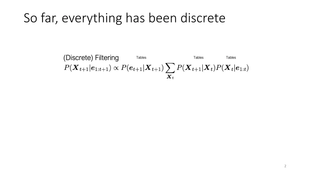
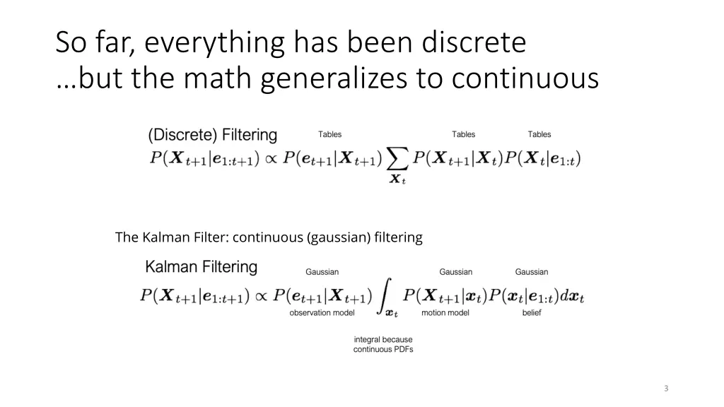
3. So far, everything has been discrete …but the math generalizes to continuous The Kalman Filter: continuous (gaussian) filtering 3

4. Think of our 2D Motion + GPS example from earlier • How do we compute the “uncertainty” on each? 4

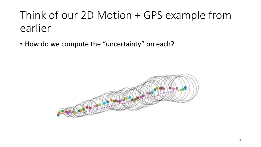
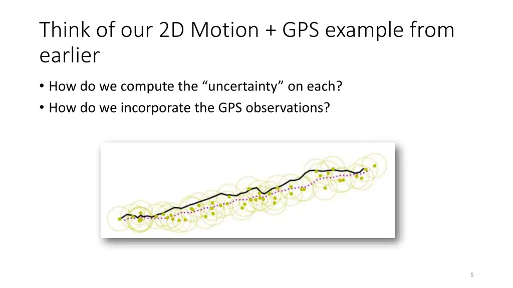
5. Think of our 2D Motion + GPS example from earlier • How do we compute the “uncertainty” on each? • How do we incorporate the GPS observations? 5

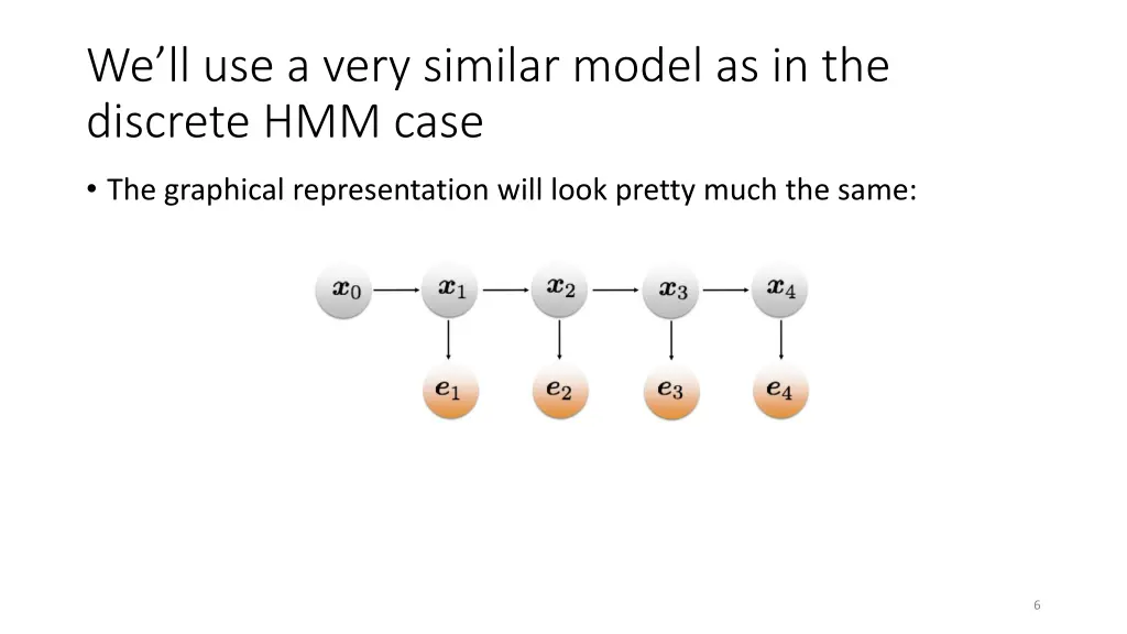
6. We’ll use a very similar model as in the discrete HMM case • The graphical representation will look pretty much the same: 6

7. Let’s start with an example in 1D • My robot moves along the x-axis: 7

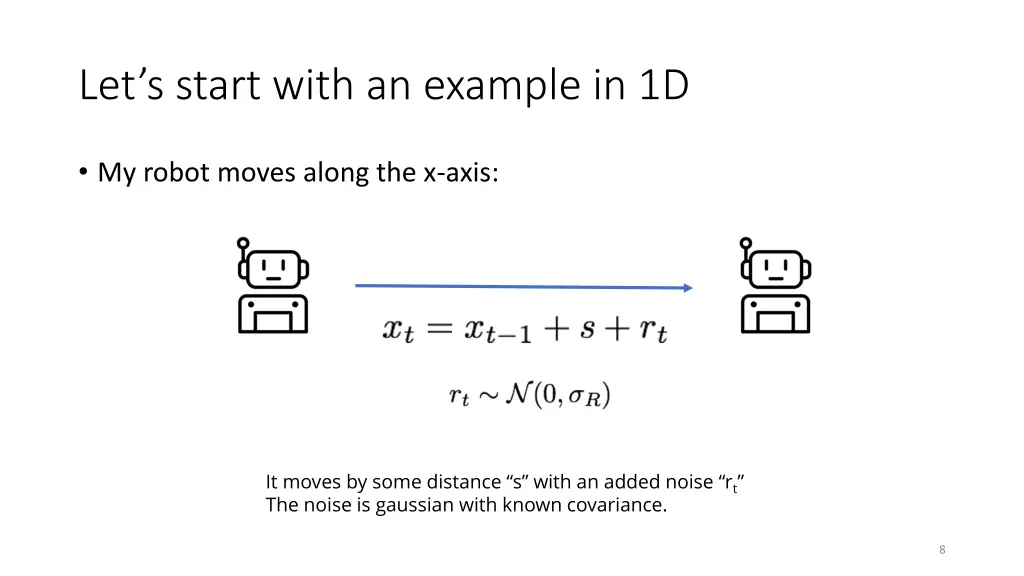
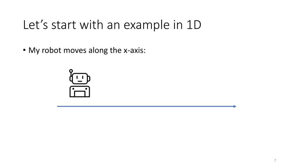
8. Let’s start with an example in 1D • My robot moves along the x-axis: It moves by some distance “s” with an added noise “rt” The noise is gaussian with known covariance. 8

9. Let’s start with an example in 1D • My robot moves along the x-axis: The motion model is therefore as follows: 9

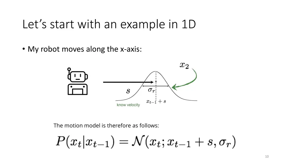
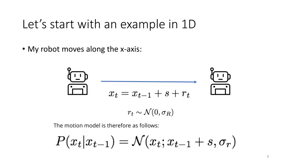
10. Let’s start with an example in 1D • My robot moves along the x-axis: The motion model is therefore as follows: 10

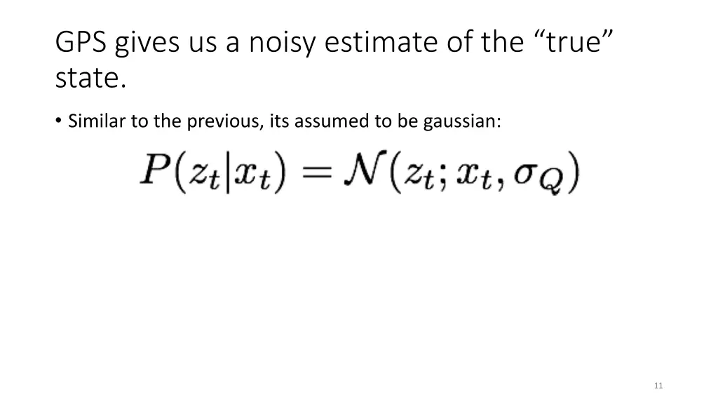
11. GPS gives us a noisy estimate of the “true” state. • Similar to the previous, its assumed to be gaussian: 11

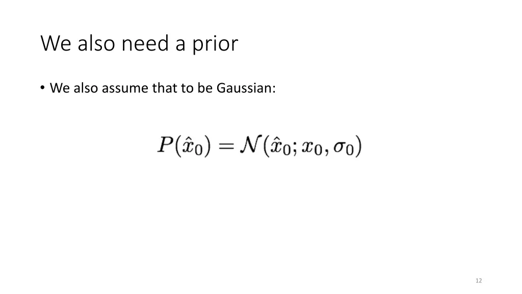
12. We also need a prior • We also assume that to be Gaussian: 12

13. Combining all these is pretty straightforward, using our model from before 13

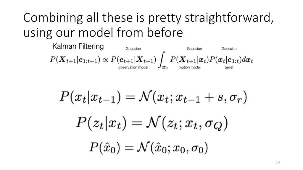
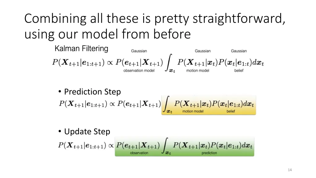
14. Combining all these is pretty straightforward, using our model from before • Prediction Step • Update Step 14

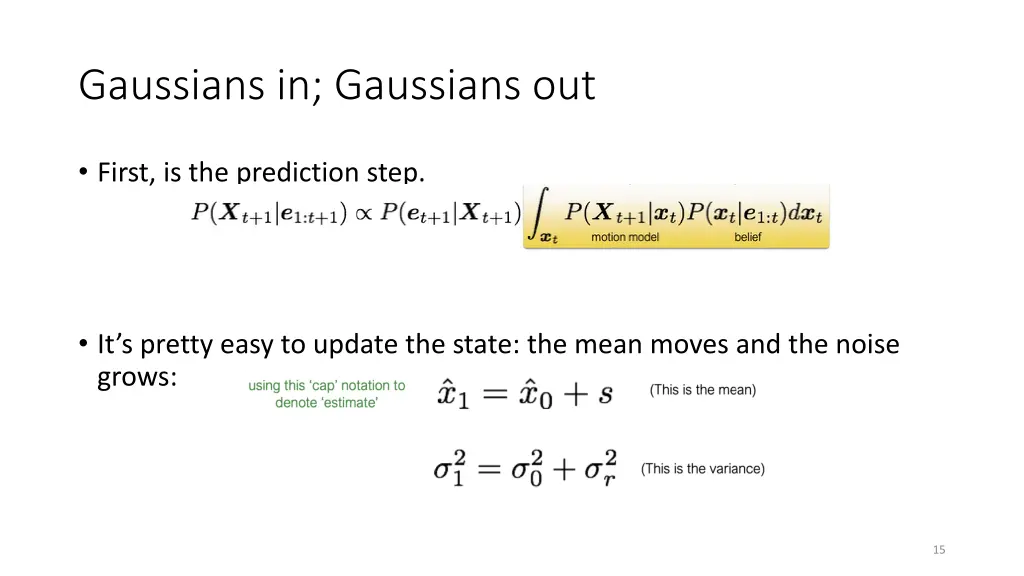
15. Gaussians in; Gaussians out • First, is the prediction step. • It’s pretty easy to update the state: the mean moves and the noise grows: 15

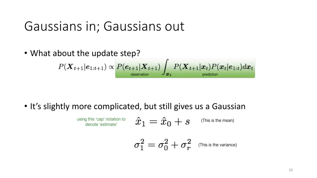
16. Gaussians in; Gaussians out • What about the update step? • It’s slightly more complicated, but still gives us a Gaussian 16

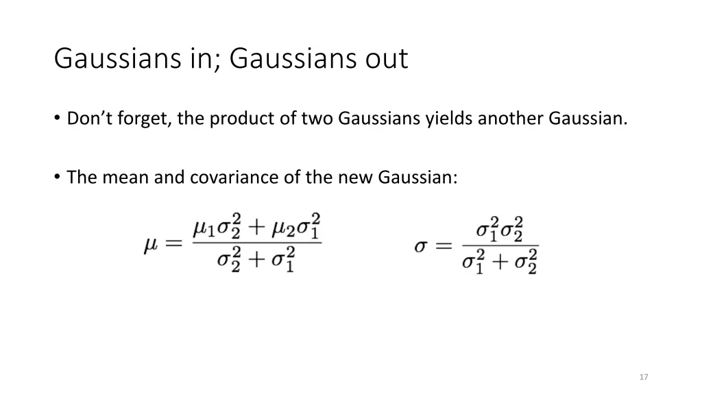
17. Gaussians in; Gaussians out • Don’t forget, the product of two Gaussians yields another Gaussian. • The mean and covariance of the new Gaussian: 17

18. Applying that Gaussian rule to the Filtering equation gives us the following: 18

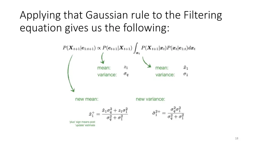
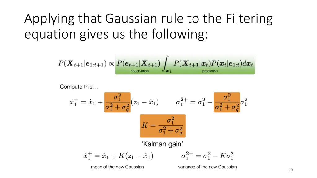
19. Applying that Gaussian rule to the Filtering equation gives us the following: 19

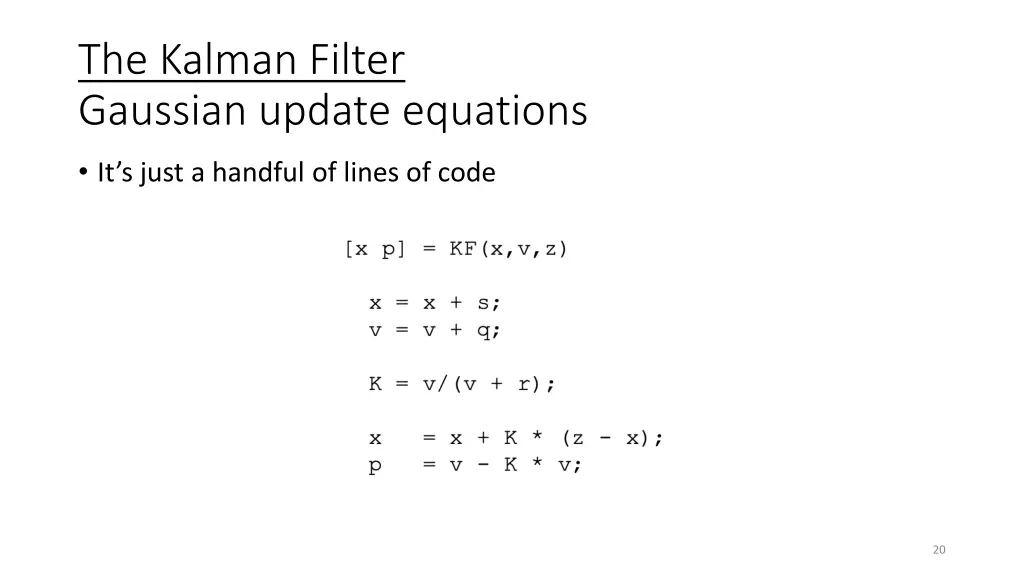
20. The Kalman Filter Gaussian update equations • It’s just a handful of lines of code 20

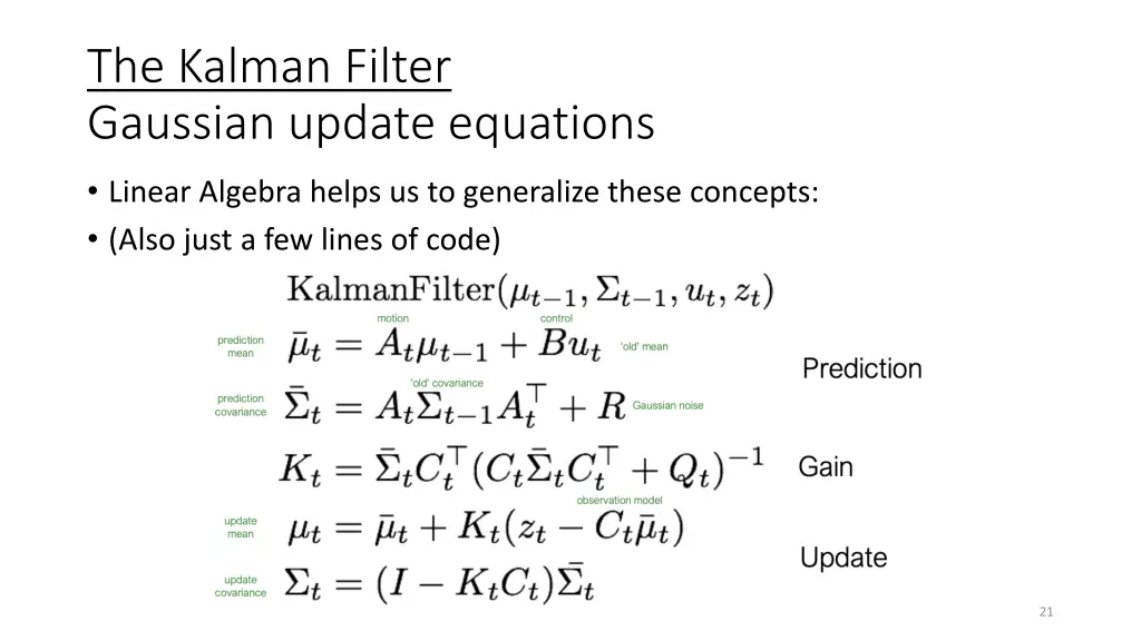
21. The Kalman Filter Gaussian update equations • Linear Algebra helps us to generalize these concepts: • (Also just a few lines of code) 21

22. Let’s revisit our 2D GPS model Does all the behavior make sense? • What are the equations the govern the motion? • Motion Model: - We are given a measurement of the movement “s” at each time step: the dx_noisy and dy_noisy - The noise is known to us: a 0.3 diagonal matrix 22

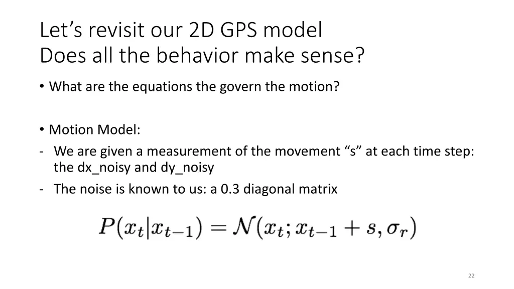
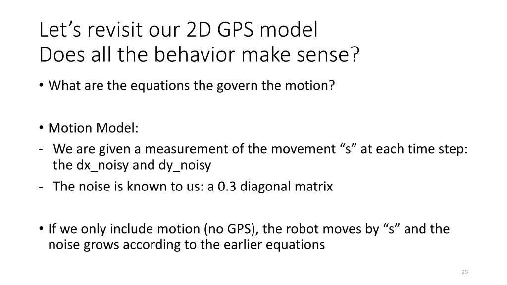
23. Let’s revisit our 2D GPS model Does all the behavior make sense? • What are the equations the govern the motion? • Motion Model: - We are given a measurement of the movement “s” at each time step: the dx_noisy and dy_noisy - The noise is known to us: a 0.3 diagonal matrix • If we only include motion (no GPS), the robot moves by “s” and the noise grows according to the earlier equations 23

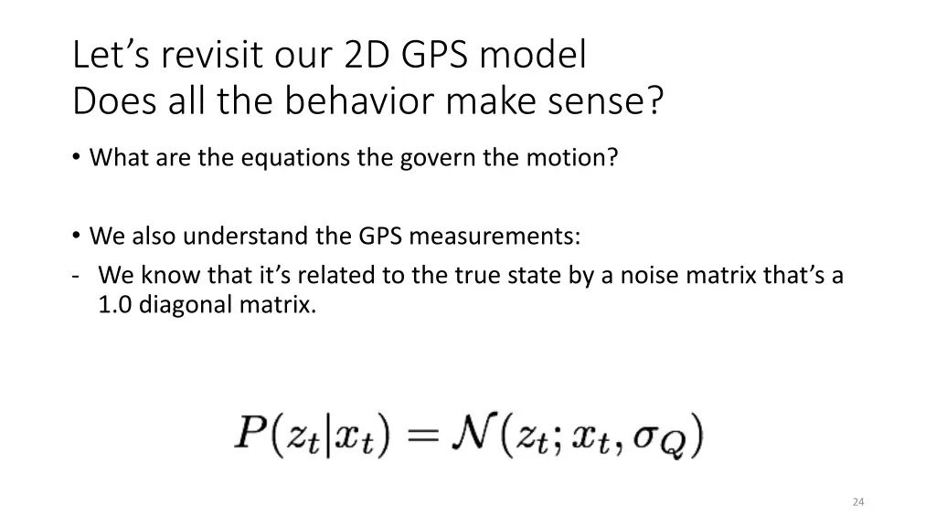
24. Let’s revisit our 2D GPS model Does all the behavior make sense? • What are the equations the govern the motion? • We also understand the GPS measurements: - We know that it’s related to the true state by a noise matrix that’s a 1.0 diagonal matrix. 24

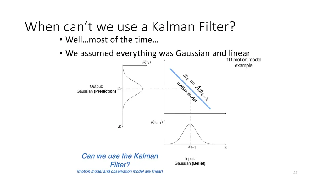
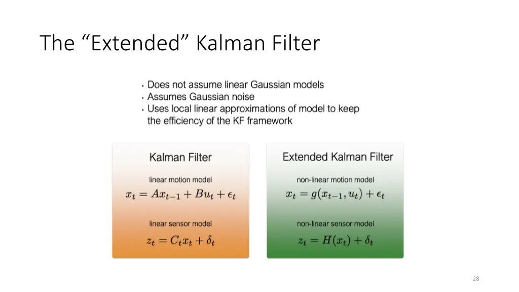
25. When can’t we use a Kalman Filter? • Well…most of the time… • We assumed everything was Gaussian and linear 25

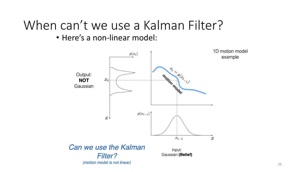
26. When can’t we use a Kalman Filter? • Here’s a non-linear model: 26

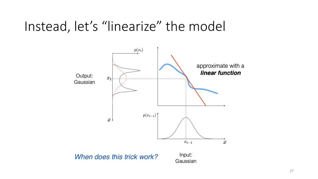
27. Instead, let’s “linearize” the model 27

28. The “Extended” Kalman Filter 28

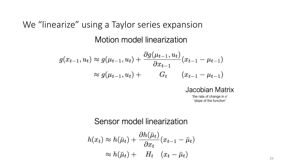
29. We “linearize” using a Taylor series expansion 29

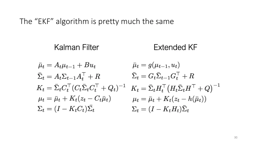
30. The “EKF” algorithm is pretty much the same 30

31. The EKF is necessary when we have a robot with orientation • If we have uncertainty in yaw, the motion model becomes nonlinear: From: https://cs.gmu.edu/%7Ekosecka/cs685/cs685-11-sensor-motion-models.pdf 31

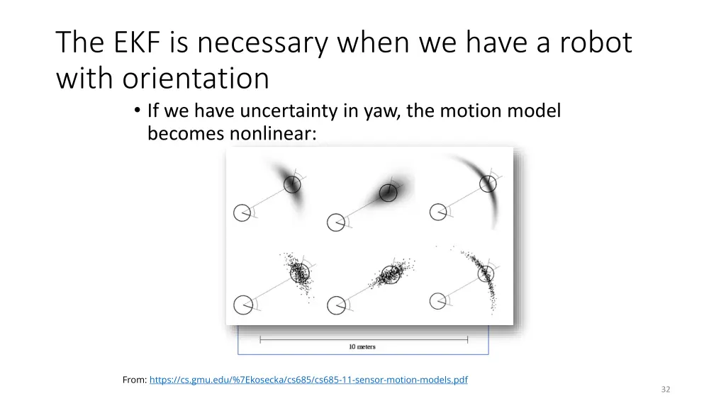
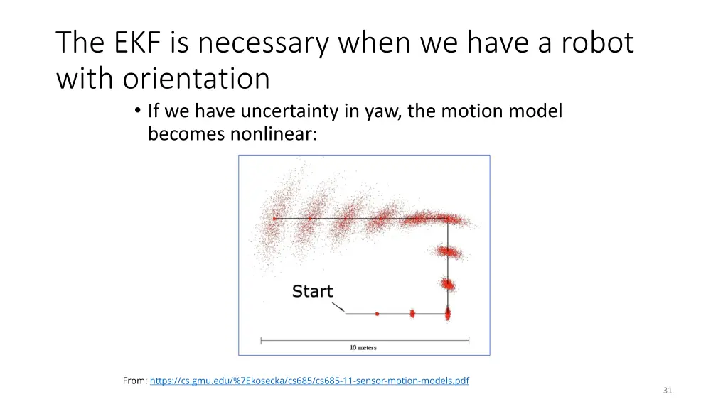
32. The EKF is necessary when we have a robot with orientation • If we have uncertainty in yaw, the motion model becomes nonlinear: From: https://cs.gmu.edu/%7Ekosecka/cs685/cs685-11-sensor-motion-models.pdf 32

33. Will the EKF help us with the “Doors” example from earlier? 33

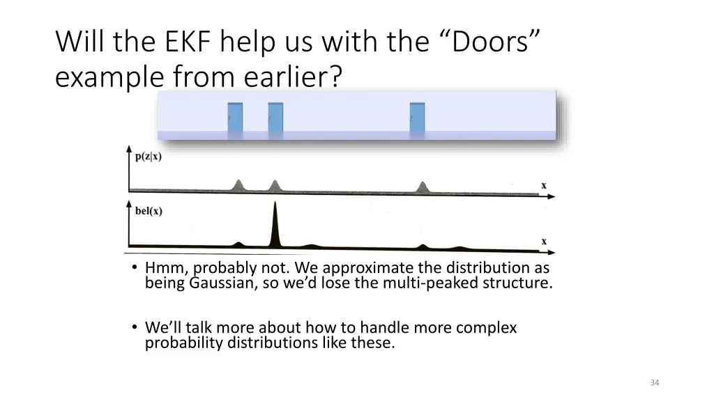
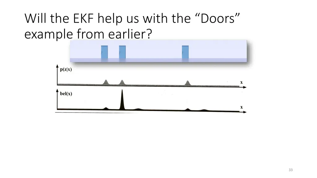
34. Will the EKF help us with the “Doors” example from earlier? • Hmm, probably not. We approximate the distribution as being Gaussian, so we’d lose the multi-peaked structure. • We’ll talk more about how to handle more complex probability distributions like these. 34

35. Let’s revisit the idea of probability distributions being represented as graphs • The graph is a convenient visual tool, but an incredibly powerful way to think about these problems more generally: • What if I removed an observation? • What if I added additional observations and sensors? 35

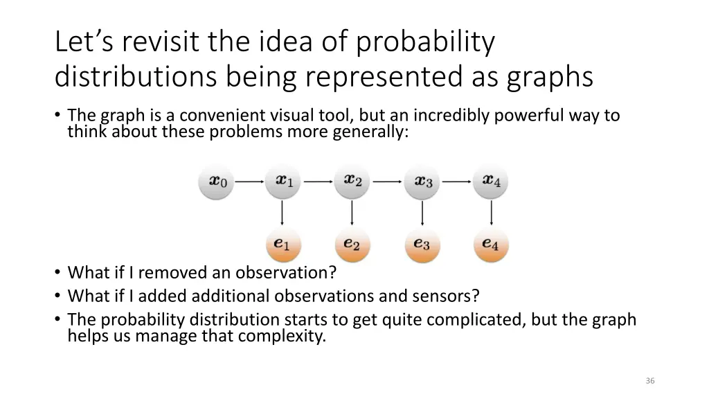
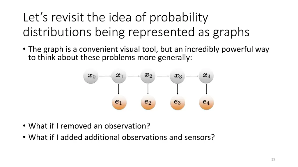
36. Let’s revisit the idea of probability distributions being represented as graphs • The graph is a convenient visual tool, but an incredibly powerful way to think about these problems more generally: • What if I removed an observation? • What if I added additional observations and sensors? • The probability distribution starts to get quite complicated, but the graph helps us manage that complexity. 36

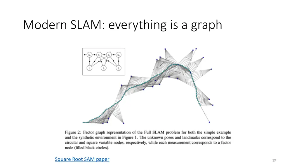
37. Modern SLAM: everything is a graph • SLAM: Simultaneous Localization and Mapping Square Root SAM paper 37

38. Modern SLAM: everything is a graph Square Root SAM paper 38

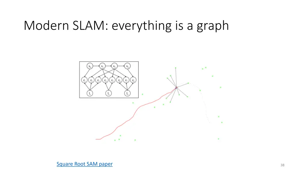
39. Modern SLAM: everything is a graph Square Root SAM paper 39